tvsews

tvsews is an R package that provides code and data for a whole-lake fertilization experiment that caused an algal bloom in order to compared the performance of early warning statistics (EWS) in temporal and spatial data.

Installation

You can install tvsews from GitHub with:

# install.packages("devtools")
devtools::install_github("cbuelo/tvsews")

To install the package and build a vignette that carries out analyses and displays results for an accepted manuscript (note this will take a few minutes to run):

devtools::install_github("cbuelo/tvsews", build_vignettes = T)
library(tvsews)
vignette("TvS-AlgalBloom-EWS")

Example

Example results from most recent experiment:

Set up and visualize time series data

library(tvsews)
library(dplyr)
library(ggplot2)
ex_data <- ts_data %>%
  filter(Year >= 2018) %>%
  select(Lake, Year, DOY, BGA_HYLB)

ex_bloom_fert_dates <- bloom_fert_dates %>%
  filter(Year >= 2018 & Lake == "R")

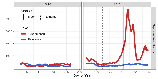
plot_state_vars(
  time_series = ex_data,
  bloom_fert_df = ex_bloom_fert_dates,
  var_rename_vec = c(`Phycocyanin (cells/mL)` = "BGA_HYLB"),
  legend_location = c(0.18, 0.7)
)

Calculate rolling window statistics and quickest detection alarms

ex_rw_stats <- calc_rolling_stats(
  data = ex_data,
  var_cols = "BGA_HYLB",
  widths = c(21)
) # warnings are missing data, okay
ex_qd_all <- run_qd(
  rolling_window_stats = ex_rw_stats,
  var_cols = "BGA_HYLB",
  widths = c(21),
  stats_to_qd = c("SD", "Ar1"),
  exp_lakes = c("R"),
  ref_lake = "L",
  ar1_alarm_rho = 0.95
)
#> [1] "Current variable QD-ing: BGA_HYLB"
ex_qd_formatted <- format_qd(
  qd_stats = ex_qd_all,
  var_cols = c("BGA_HYLB")
)

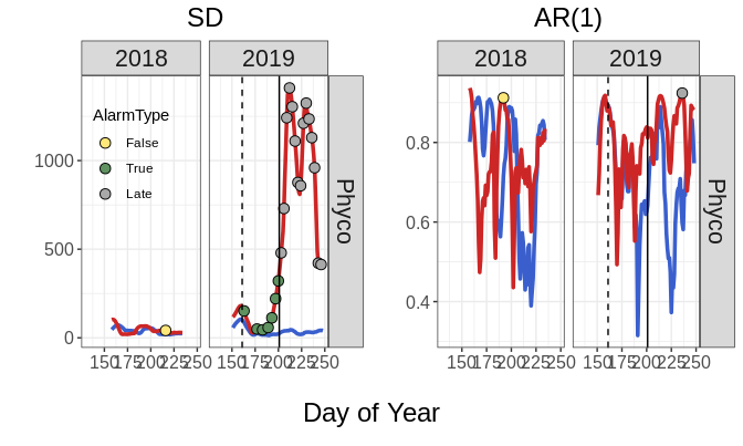
# plot the rolling window statistics and alarms
time_series_plot <- plot_temporal_EWS(
  rolling_window_stats = ex_rw_stats,
  qd_alarms = ex_qd_formatted,
  bloom_fert_df = ex_bloom_fert_dates,
  var_rename_vec = c(`Phyco` = "BGA_HYLB"),
  legend_location = c(0.2, 0.7)
)

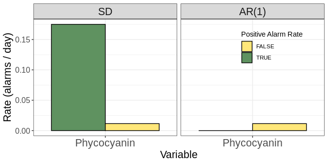
Calculate and plot true and false alarm rates

alarm_rates <- calc_alarm_rates(
  qd_alarms = ex_qd_formatted,
  bloom_fert_df = bloom_fert_dates
)

plot_alarm_rates(
  qd_alarm_rates = alarm_rates,
  var_rename_vec = c("Phycocyanin" = "BGA_HYLB"),
  legend_title = "Positive Alarm Rate"
)

Plot example spatial data

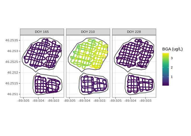
plot_spatial_data(
  spatial_data = flame_data,
  samples_to_plot = data.frame(Year = 2019, DOY = c(165, 210, 228), stringsAsFactors = FALSE),
  var_cols = c("BGApc_ugL_tau")
)

Calculate spatial statistics

Just dates in pre-bloom fertilization period to limit computation time.

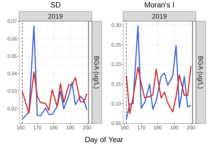
ex_spatial_data_pbfp <- flame_data %>%
  filter(Year == 2019 & between(DOY, 161, 201))

spatial_stats_pbfp <- calc_spatial_stats(
  spatial_data = ex_spatial_data_pbfp,
  var_cols = c("BGApc_ugL_tau")
) # ignore estimated time as not using all of default data

Plot spatial statistics

spatial_results_plot <- plot_spatial_EWS(spatial_stats_pbfp)

(Note to self: devtools::build_readme()to render)