A comprehensive tool to infer TF-centered, spatial gene regulatory networks for the spatially resolved transcriptomics (SRT) data.
SpaGRN is an open-source Python package for inferring gene regulatory networks (GRNs) based on spatial gene expression data using GPLv3 license. The model takes into account the spatial proximity of genes and TF binding to infer their regulatory relationships. The package is particularly useful for analyzing spatially resolved gene expression data.
RRID: SCR_023451
we provide two modules to infer the co-expressed and co-localized gene network:
- spatially-aware cross-correlation (SCC) model
- spatial-proximity-graph (SPG) model
- Stereo-seq Mouse Brain
- Stereo-seq Drosophila Embryo and Larvae
All input SRT data and related TF database can be inquired or directly downloaded from http://www.bgiocean.com/SpaGRN/ We also provide an interactive 3D GRN atlas database, covering different GRN inference tools for different SRT datasets generated by different SRT sequencing platforms (http://www.bgiocean.com/SpaGRN/).
To install the latest version of SpaGRN via PyPI:
pip install spagrn==1.0.7
Or install by bioconda
conda install -c bioconda spagrn

# Notice: If you install via conda, you will need to install the following dependencies separately:
#pyscenic==0.12.1
#hotspotsc==1.1.1
#arboreto
#ctxcore>=0.2.0
SpaGRN can be imported as:
from spagrn import InferNetwork as irn
from spagrn import plot as prn
Dependencies:
anndata==0.8.0
pandas<2.0.0,>=1.3.4
scanpy==1.9.1
seaborn
matplotlib
pyscenic==0.12.1
hotspotsc==1.1.1
scipy
numpy
dask
arboreto
ctxcore>=0.2.0
scikit-learn
The package provides functions for loading data, preprocessing data, reconstructing gene network, and visualizing the inferred GRNs. The main functions are:
- Load and process data
- Compute TF-gene similarities
- Create modules
- Perform motif enrichment and determine regulons
- Calculate regulon activity level across cells
- Visualize network and other results
from spagrn import InferRegulatoryNetwork as irn

if __name__ == '__main__':  #notice: to avoid concurrent bugs, please do not ignore this line!
    database_fn='mouse.feather'
    motif_anno_fn='mouse.tbl'
    tfs_fn='mouse_TFs.txt'
    # load Ligand-receptor data
    niches = pd.read_csv('niches.csv')
    # Load data
    data = irn.read_file('data.h5ad')
    # Preprocess data
    data = irn.preprocess(data)
    # Initialize gene regulatory network
    grn = irn(data)
    # run main pipeline
    grn.infer(database_fn,
              motif_anno_fn,
              tfs_fn,
              niche_df=niches,
              num_workers=cpu_count(),
              cache=False,
              save_tmp=True,
              c_threshold=0.2,
              layers=None,
              latent_obsm_key='spatial',
              model='danb',
              n_neighbors=30,
              weighted_graph=False,
              cluster_label='celltype',
              method='spg',
              prefix='project',
              noweights=False)
All results will be save in a h5ad file, default file name is spagrn.h5ad.
SpaGRN offers a wide range of data visualization methods.
# read data from previous analysis
data = irn.read_file('spagrn.h5ad')
auc_mtx = data.obsm['auc_mtx']

# plot
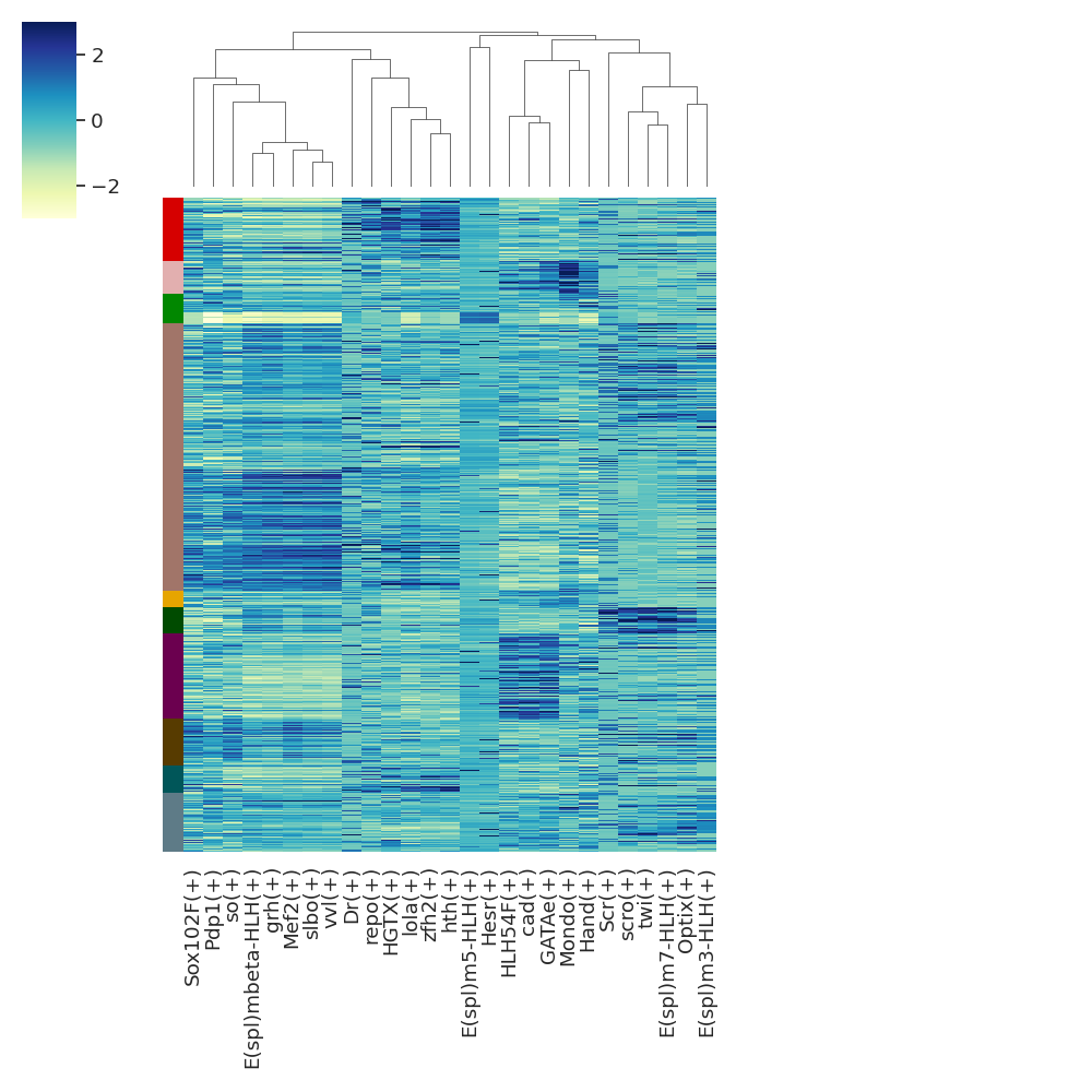
prn.auc_heatmap(data,
                auc_mtx,
                cluster_label='annotation',
                rss_fn='regulon_specificity_scores.txt',
                topn=10,
                subset=False,
                save=True,
                fn='clusters_heatmap_top10.pdf',
                legend_fn="rss_celltype_legend_top10.pdf")
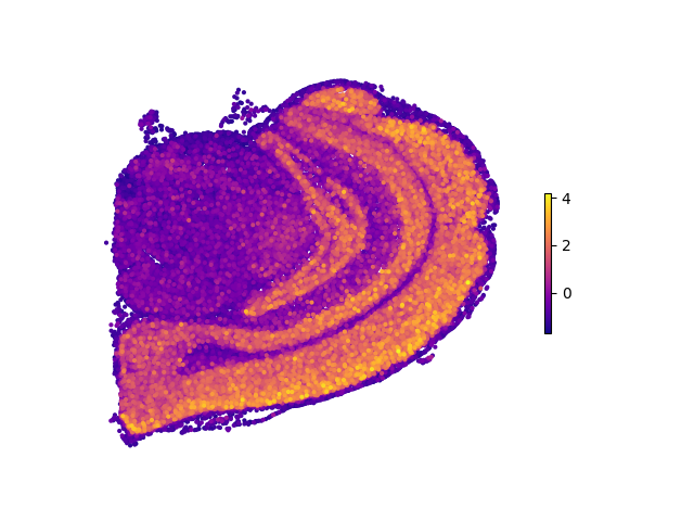
Plot spatial distribution map of a regulon on a 2D plane:
from spagrn import plot as prn

prn.plot_2d_reg(data, 'spatial', auc_mtx, reg_name='Egr3')
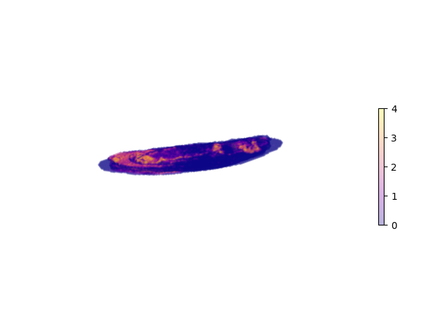
If one wants to display their 3D data in a three-dimensional fashion:
prn.plot_3d_reg(data, 'spatial', auc_mtx, reg_name='grh', vmin=0, vmax=4, alpha=0.3)


