TIGER
Introduction
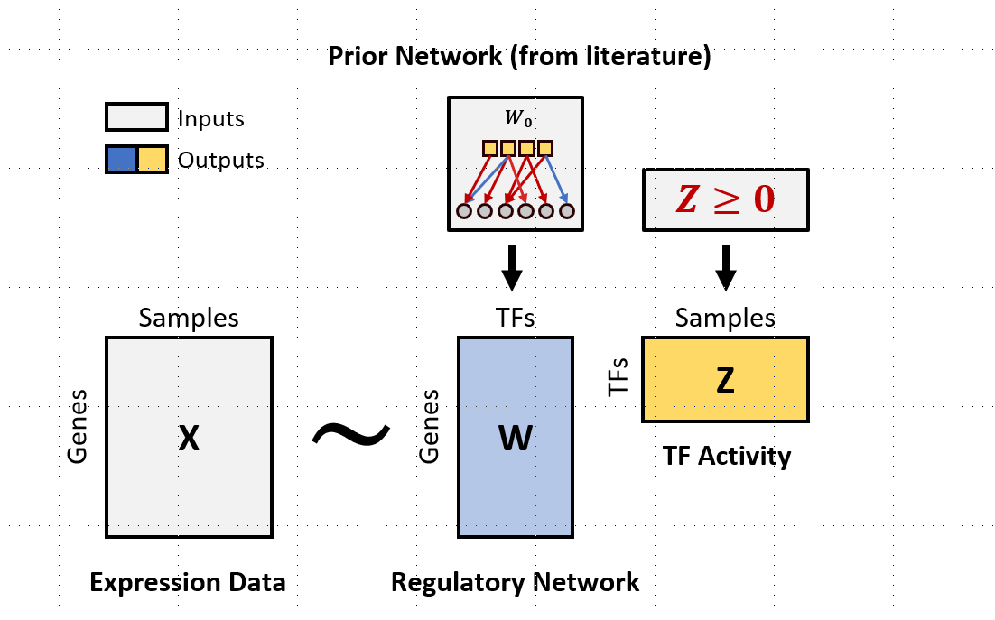
The goal of TIGER is to estimate gene regulatory network and
transcription factor activities using Bayesian matrix factorization.

Please read and cite the following article when you use TIGER:
Joint inference of transcription factor activity and context-specific
regulatory networks, Chen&Padi
2022
Installation
TIGER relies on cmdstanr for Beyesian Inference. You can install the latest beta release of the cmdstanr R package with
install.packages("cmdstanr", repos = c("https://mc-stan.org/r-packages/", getOption("repos")))Then, you can use cmdstanr to install CmdStan, the shell interface to Stan with
cmdstanr::install_cmdstan()These two steps are usually enough if your C++ toolchain is set up properly. For example, use RTools 4.0 toolchain which contains a g++ 8 compiler and mingw32-make on Windows platform. If you see problems with installation, you can go to cmdstanr installation for more information.
After cmdstan is correctly installed, you can install the development version of TIGER with:
devtools::install_github("cchen22/TIGER")Quick start
This is a simple example of TIGER on a small dataset. TIGER requires two inputs -
- a normalized expression matrix with rows as genes and column as samples;
- a prior network with rows as TFs and column as genes. The network is signed and binarized (e.g., -1,0,1).
library(TIGER)

##1. load data
expr = TIGER::expr
prior = TIGER::prior

##2. run TIGER with default parameters
ss = TIGER(expr,prior)
## Estimating optimal shrinkage intensity lambda (correlation matrix): 0.6787
##
## ------------------------------------------------------------
## EXPERIMENTAL ALGORITHM:
## This procedure has not been thoroughly tested and may be unstable
## or buggy. The interface is subject to change.
## ------------------------------------------------------------
## Gradient evaluation took 0.003798 seconds
## 1000 transitions using 10 leapfrog steps per transition would take 37.98 seconds.
## Adjust your expectations accordingly!
## Begin eta adaptation.
## Iteration: 1 / 250 [ 0%] (Adaptation)
## Iteration: 50 / 250 [ 20%] (Adaptation)
## Iteration: 100 / 250 [ 40%] (Adaptation)
## Iteration: 150 / 250 [ 60%] (Adaptation)
## Iteration: 200 / 250 [ 80%] (Adaptation)
## Iteration: 250 / 250 [100%] (Adaptation)
## Success! Found best value [eta = 0.1].
## Begin stochastic gradient ascent.
## iter ELBO delta_ELBO_mean delta_ELBO_med notes
## 100 -1171074.398 1.000 1.000
## 200 -157823.051 3.710 6.420
## 300 -75833.770 2.834 1.081
## 400 -58183.111 2.201 1.081
## 500 -53081.533 1.780 1.000
## 600 -51050.359 1.490 1.000
## 700 -49850.082 1.281 0.303
## 800 -49097.595 1.123 0.303
## 900 -48638.556 0.999 0.096
## 1000 -48219.092 0.900 0.096
## 1100 -47906.769 0.819 0.040 MAY BE DIVERGING... INSPECT ELBO
## 1200 -47734.081 0.751 0.040 MAY BE DIVERGING... INSPECT ELBO
## 1300 -47557.680 0.693 0.024 MAY BE DIVERGING... INSPECT ELBO
## 1400 -47412.426 0.644 0.024 MAY BE DIVERGING... INSPECT ELBO
## 1500 -47351.151 0.601 0.015 MAY BE DIVERGING... INSPECT ELBO
## 1600 -47269.802 0.564 0.015 MAY BE DIVERGING... INSPECT ELBO
## 1700 -47192.708 0.531 0.009 MAY BE DIVERGING... INSPECT ELBO
## 1800 -47166.698 0.501 0.009 MAY BE DIVERGING... INSPECT ELBO
## 1900 -47082.350 0.475 0.009
## 2000 -47084.804 0.451 0.009
## 2100 -47043.676 0.430 0.007
## 2200 -47003.345 0.410 0.007
## 2300 -46991.764 0.392 0.004 MEDIAN ELBO CONVERGED
## Drawing a sample of size 300 from the approximate posterior...
## COMPLETED.
## Finished in 35.4 seconds.
##3. print the TFA score in first three samples
tgres = ss$Z
tgres[,1:3]
## GSM782710_CEBPD GSM782711_CEBPZ GSM782714_ETS1
## CEBPD 0.16995715 0.06962729 0.07757839
## CEBPZ 0.04584281 0.01014883 0.10245526
## ETS1 0.10160440 0.09648879 0.02618637
## FOXM1 0.53454111 0.15332452 0.19762255
## FOXO3 0.18207905 0.16695081 0.17561871
## HSF2 0.08228031 0.03063709 0.13700934
## MITF 0.15515221 0.13553729 0.12691376
## RELA 0.10513991 0.08928370 0.03607522
## SP1 0.04577883 0.03665489 0.09852019
## SP100 0.04896814 0.06436493 0.04137325
## STAT1 0.04235073 0.04073346 0.05757398
## STAT3 0.09059502 0.08443980 0.04378273
## STAT6 0.13057221 0.17615136 0.09388253
## TP53 0.04618498 0.04375639 0.07959729
Wokring with DoRothEA prior
TIGER provides some convenient functions to work with DoRothEA prior database. Firstly, install DoRothEA R package from Bioconductor
BiocManager::install("dorothea")DoRothEA provides regulons for two species - human and mouse. For example,if we have a human cancer expression matrix and want to estimate the TFA in each cancer sample, then we can use the following code to prepare the prior network.
## load dorothea pancancer database
df = dorothea::dorothea_hs_pancancer

## convert it to TIGER prior format (e.g., adjacency matrix)
prior = el2adj(df[,-2])