AI-text-to-video-model-from-scratch: A Jupyter Notebook repository from cenphoenix

Building AI Text to Video Model From Scratch Using Python

Sora from OpenAI, Stable Video Diffusion from Stability AI, and many other text-to-video models that have come out or will appear in the future are among the most popular AI trends in 2024, following large language models (LLMs). In this blog, we will build a small scale text-to-video model from scratch. We will input a text prompt, and our trained model will generate a video based on that prompt. This blog will cover everything from understanding the theoretical concepts to coding the entire architecture and generating the final result.

Since I don’t have a fancy GPU, I’ve coded the small-scale architecture. Here’s a comparison of the time required to train the model on different processors:

Training Videos	Epochs	CPU	GPU A10	GPU T4
10K	30	more than 3 hr	1 hr	1 hr 42m
30K	30	more than 6 hr	1 hr 30	2 hr 30
100K	30	-	3-4 hr	5-6 hr

Running on a CPU will obviously take much longer to train the model. If you need to quickly test changes in the code and see results, CPU is not the best choice. I recommend using a T4 GPU from Colab or Kaggle for more efficient and faster training.

Here is the blog link which guides you on how to create Stable Diffusion from scratch: Coding Stable Diffusion from Scratch

What We’re Building
Prerequisites
Understanding the GAN Architecture
Setting the Stage
Coding the Training Data
Pre-Processing Our Training Data
Implementing Text Embedding Layer
Implementing Generator Layer
Implementing Discriminator Layer
Coding Training Parameters
Coding the Training Loop
Saving the Trained Model
Generating AI Video
What’s Missing?
About Me

What We’re Building

We will follow a similar approach to traditional machine learning or deep learning models that train on a dataset and are then tested on unseen data. In the context of text-to-video, let’s say we have a training dataset of 100K videos of dogs fetching balls and cats chasing mice. We will train our model to generate videos of a cat fetching a ball or a dog chasing a mouse.

Although such training datasets are easily available on the internet, the required computational power is extremely high. Therefore, we will work with a video dataset of moving objects generated from Python code.

We will use the GAN (Generative Adversarial Networks) architecture to create our model instead of the diffusion model that OpenAI Sora uses. I attempted to use the diffusion model, but it crashed due to memory requirements, which is beyond my capacity. GANs, on the other hand, are easier and quicker to train and test.

Prerequisites

We will be using OOP (Object-Oriented Programming), so you must have a basic understanding of it along with neural networks. Knowledge of GANs (Generative Adversarial Networks) is not mandatory, as we will be covering their architecture here.

Topic	Link
OOP	Video Link
Neural Networks Theory	Video Link
GAN Architecture	Video Link
Python basics	Video Link

Understanding the GAN Architecture

Understanding GAN architecture is important because much of our architecture depends on it. Let’s explore what it is, its components, and more.

what is GAN?

Generative Adversarial Network (GAN) is a deep learning model where two neural networks compete: one creates new data (like images or music) from a given dataset, and the other tries to tell if the data is real or fake. This process continues until the generated data is indistinguishable from the original.

Real-World Application

Generate Images: GANs create realistic images from text prompts or modify existing images, such as enhancing resolution or adding color to black-and-white photos.
Data Augmentation: They generate synthetic data to train other machine learning models, such as creating fraudulent transaction data for fraud detection systems.
Complete Missing Information: GANs can fill in missing data, like generating sub-surface images from terrain maps for energy applications.
Generate 3D Models: They convert 2D images into 3D models, useful in fields like healthcare for creating realistic organ images for surgical planning.

How does a GAN work?

It consists of two deep neural networks: the generator and the discriminator. These networks train together in an adversarial setup, where one generates new data and the other evaluates if the data is real or fake.

Here’s a simplified overview of how GAN works:

Training Set Analysis: The generator analyzes the training set to identify data attributes, while the discriminator independently analyzes the same data to learn its attributes.
Data Modification: The generator adds noise (random changes) to some attributes of the data.
Data Passing: The modified data is then passed to the discriminator.
Probability Calculation: The discriminator calculates the probability that the generated data is from the original dataset.
Feedback Loop: The discriminator provides feedback to the generator, guiding it to reduce random noise in the next cycle.
Adversarial Training: The generator tries to maximize the discriminator’s mistakes, while the discriminator tries to minimize its own errors. Through many training iterations, both networks improve and evolve.
Equilibrium State: Training continues until the discriminator can no longer distinguish between real and synthesized data, indicating that the generator has successfully learned to produce realistic data. At this point, the training process is complete.

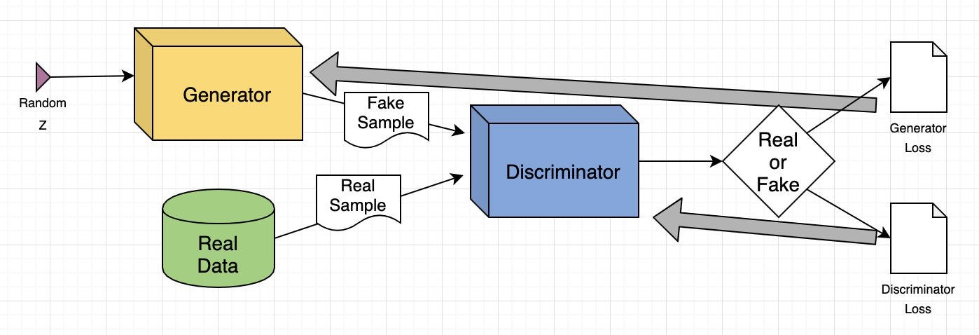
image from aws guide

GAN training example

Let’s explain the GAN model with an example of image-to-image translation, focusing on modifying a human face.

Input Image: The input is a real image of a human face.
Attribute Modification: The generator modifies attributes of the face, like adding sunglasses to the eyes.
Generated Images: The generator creates a set of images with sunglasses added.
Discriminator’s Task: The discriminator receives a mix of real images (people with sunglasses) and generated images (faces where sunglasses were added).
Evaluation: The discriminator tries to differentiate between real and generated images.
Feedback Loop: If the discriminator correctly identifies fake images, the generator adjusts its parameters to produce more convincing images. If the generator successfully fools the discriminator, the discriminator updates its parameters to improve its detection.

Through this adversarial process, both networks continuously improve. The generator gets better at creating realistic images, and the discriminator gets better at identifying fakes until equilibrium is reached, where the discriminator can no longer tell the difference between real and generated images. At this point, the GAN has successfully learned to produce realistic modifications.

Setting the Stage

Installing the required libraries is the first step in building our text-to-video model.

pip install -r requirements.txt

We will be working with a range of Python libraries, Let’s import them.

# Operating System module for interacting with the operating system
import os

# Module for generating random numbers
import random

# Module for numerical operations
import numpy as np

# OpenCV library for image processing
import cv2

# Python Imaging Library for image processing
from PIL import Image, ImageDraw, ImageFont

# PyTorch library for deep learning
import torch

# Dataset class for creating custom datasets in PyTorch
from torch.utils.data import Dataset

# Module for image transformations
import torchvision.transforms as transforms

# Neural network module in PyTorch
import torch.nn as nn

# Optimization algorithms in PyTorch
import torch.optim as optim

# Function for padding sequences in PyTorch
from torch.nn.utils.rnn import pad_sequence

# Function for saving images in PyTorch
from torchvision.utils import save_image

# Module for plotting graphs and images
import matplotlib.pyplot as plt

# Module for displaying rich content in IPython environments
from IPython.display import clear_output, display, HTML

# Module for encoding and decoding binary data to text
import base64

Now that we’ve imported all of our libraries, the next step is to define our training data that we will be using to train our GAN architecture.

Coding the Training Data

We need to have at least 10,000 videos as training data. Why? Well, because I tested with smaller numbers and the results were very poor, practically nothing to see. The next big question is: what are these videos about? Our training video dataset consists of a circle moving in different directions with different motions. So, let’s code it and generate 10,000 videos to see what it looks like.

# Create a directory named 'training_dataset'
os.makedirs('training_dataset', exist_ok=True)

# Define the number of videos to generate for the dataset
num_videos = 10000

# Define the number of frames per video (1 Second Video)
frames_per_video = 10

# Define the size of each image in the dataset
img_size = (64, 64)

# Define the size of the shapes (Circle)
shape_size = 10

after settings some basic parameters next we need to define the text prompts of our training dataset based on which training videos will be generated.

# Define text prompts and corresponding movements for circles
prompts_and_movements = [
    ("circle moving down", "circle", "down"),  # Move circle downward
    ("circle moving left", "circle", "left"),  # Move circle leftward
    ("circle moving right", "circle", "right"),  # Move circle rightward
    ("circle moving diagonally up-right", "circle", "diagonal_up_right"),  # Move circle diagonally up-right
    ("circle moving diagonally down-left", "circle", "diagonal_down_left"),  # Move circle diagonally down-left
    ("circle moving diagonally up-left", "circle", "diagonal_up_left"),  # Move circle diagonally up-left
    ("circle moving diagonally down-right", "circle", "diagonal_down_right"),  # Move circle diagonally down-right
    ("circle rotating clockwise", "circle", "rotate_clockwise"),  # Rotate circle clockwise
    ("circle rotating counter-clockwise", "circle", "rotate_counter_clockwise"),  # Rotate circle counter-clockwise
    ("circle shrinking", "circle", "shrink"),  # Shrink circle
    ("circle expanding", "circle", "expand"),  # Expand circle
    ("circle bouncing vertically", "circle", "bounce_vertical"),  # Bounce circle vertically
    ("circle bouncing horizontally", "circle", "bounce_horizontal"),  # Bounce circle horizontally
    ("circle zigzagging vertically", "circle", "zigzag_vertical"),  # Zigzag circle vertically
    ("circle zigzagging horizontally", "circle", "zigzag_horizontal"),  # Zigzag circle horizontally
    ("circle moving up-left", "circle", "up_left"),  # Move circle up-left
    ("circle moving down-right", "circle", "down_right"),  # Move circle down-right
    ("circle moving down-left", "circle", "down_left"),  # Move circle down-left
]

We’ve defined several movements of our circle using these prompts. Now, we need to code some mathematical equations to move that circle based on the prompts.

# defining function to create image with moving shape
def create_image_with_moving_shape(size, frame_num, shape, direction):

    # Create a new RGB image with specified size and white background
    img = Image.new('RGB', size, color=(255, 255, 255))

    # Create a drawing context for the image
    draw = ImageDraw.Draw(img)

    # Calculate the center coordinates of the image
    center_x, center_y = size[0] // 2, size[1] // 2

    # Initialize position with center for all movements
    position = (center_x, center_y)

    # Define a dictionary mapping directions to their respective position adjustments or image transformations
    direction_map = {
        # Adjust position downwards based on frame number
        "down": (0, frame_num * 5 % size[1]),
        # Adjust position to the left based on frame number
        "left": (-frame_num * 5 % size[0], 0),
        # Adjust position to the right based on frame number
        "right": (frame_num * 5 % size[0], 0),
        # Adjust position diagonally up and to the right
        "diagonal_up_right": (frame_num * 5 % size[0], -frame_num * 5 % size[1]),
        # Adjust position diagonally down and to the left
        "diagonal_down_left": (-frame_num * 5 % size[0], frame_num * 5 % size[1]),
        # Adjust position diagonally up and to the left
        "diagonal_up_left": (-frame_num * 5 % size[0], -frame_num * 5 % size[1]),
        # Adjust position diagonally down and to the right
        "diagonal_down_right": (frame_num * 5 % size[0], frame_num * 5 % size[1]),
        # Rotate the image clockwise based on frame number
        "rotate_clockwise": img.rotate(frame_num * 10 % 360, center=(center_x, center_y), fillcolor=(255, 255, 255)),
        # Rotate the image counter-clockwise based on frame number
        "rotate_counter_clockwise": img.rotate(-frame_num * 10 % 360, center=(center_x, center_y), fillcolor=(255, 255, 255)),
        # Adjust position for a bouncing effect vertically
        "bounce_vertical": (0, center_y - abs(frame_num * 5 % size[1] - center_y)),
        # Adjust position for a bouncing effect horizontally
        "bounce_horizontal": (center_x - abs(frame_num * 5 % size[0] - center_x), 0),
        # Adjust position for a zigzag effect vertically
        "zigzag_vertical": (0, center_y - frame_num * 5 % size[1]) if frame_num % 2 == 0 else (0, center_y + frame_num * 5 % size[1]),
        # Adjust position for a zigzag effect horizontally
        "zigzag_horizontal": (center_x - frame_num * 5 % size[0], center_y) if frame_num % 2 == 0 else (center_x + frame_num * 5 % size[0], center_y),
        # Adjust position upwards and to the right based on frame number
        "up_right": (frame_num * 5 % size[0], -frame_num * 5 % size[1]),
        # Adjust position upwards and to the left based on frame number
        "up_left": (-frame_num * 5 % size[0], -frame_num * 5 % size[1]),
        # Adjust position downwards and to the right based on frame number
        "down_right": (frame_num * 5 % size[0], frame_num * 5 % size[1]),
        # Adjust position downwards and to the left based on frame number
        "down_left": (-frame_num * 5 % size[0], frame_num * 5 % size[1])
    }

    # Check if direction is in the direction map
    if direction in direction_map:
        # Check if the direction maps to a position adjustment
        if isinstance(direction_map[direction], tuple):
            # Update position based on the adjustment
            position = tuple(np.add(position, direction_map[direction]))
        else:  # If the direction maps to an image transformation
            # Update the image based on the transformation
            img = direction_map[direction]

    # Return the image as a numpy array
    return np.array(img)

The function above is used to move our circle for each frame based on the selected direction. We just need to run a loop on top of it up to the number of videos times to generate all videos.

# Iterate over the number of videos to generate
for i in range(num_videos):
    # Randomly choose a prompt and movement from the predefined list
    prompt, shape, direction = random.choice(prompts_and_movements)
    
    # Create a directory for the current video
    video_dir = f'training_dataset/video_{i}'
    os.makedirs(video_dir, exist_ok=True)
    
    # Write the chosen prompt to a text file in the video directory
    with open(f'{video_dir}/prompt.txt', 'w') as f:
        f.write(prompt)
    
    # Generate frames for the current video
    for frame_num in range(frames_per_video):
        # Create an image with a moving shape based on the current frame number, shape, and direction
        img = create_image_with_moving_shape(img_size, frame_num, shape, direction)
        
        # Save the generated image as a PNG file in the video directory
        cv2.imwrite(f'{video_dir}/frame_{frame_num}.png', img)

Once you run the above code, it will generate our entire training dataset. Here is what the structure of our training dataset files looks like.

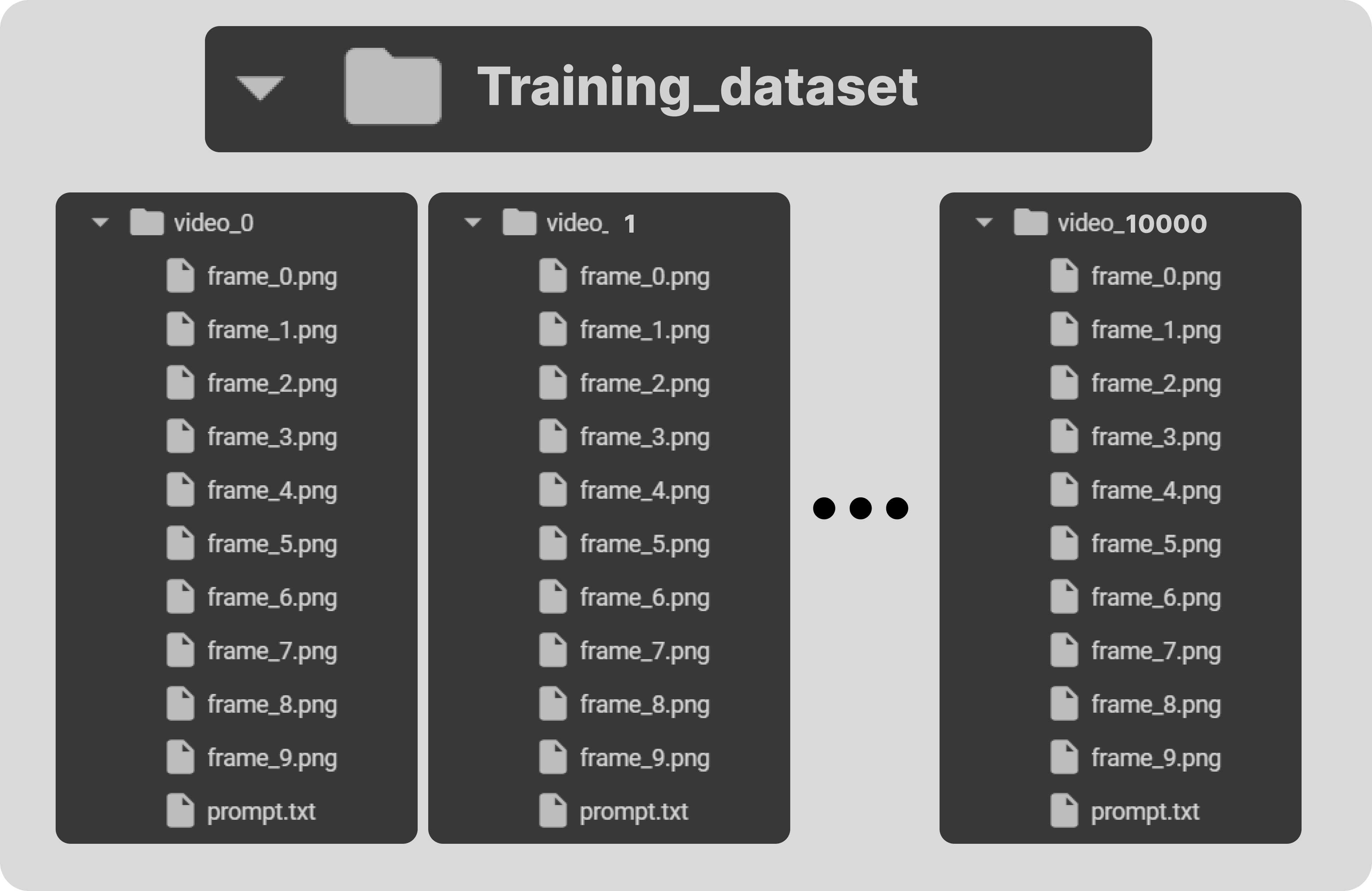
Each training video folder contains its frames along with its text prompt. Let’s take a look at the sample of our training dataset.

In our training dataset, we haven’t included the motion of the circle moving up and then to the right. We will use this as our testing prompt to evaluate our trained model on unseen data.

One more important point to note is that our training data does contains many samples where objects moving away from the scene or appear partially in front of the camera, similar to what we have observed in the OpenAI Sora demo videos.

The reason for including such samples in our training data is to test whether our model can maintain consistency when the circle enters the scene from the very corner without breaking its shape.

Now that our training data has been generated, we need to convert the training videos to tensors, which are the primary data type used in deep learning frameworks like PyTorch. Additionally, performing transformations like normalization helps improve the convergence and stability of the training architecture by scaling the data to a smaller range.

Pre-Processing Our Training Data

We have to code a dataset class for text-to-video tasks, which can read video frames and their corresponding text prompts from the training dataset directory, making them available for use in PyTorch.

# Define a dataset class inheriting from torch.utils.data.Dataset
class TextToVideoDataset(Dataset):
    def __init__(self, root_dir, transform=None):
        # Initialize the dataset with root directory and optional transform
        self.root_dir = root_dir
        self.transform = transform
        # List all subdirectories in the root directory
        self.video_dirs = [os.path.join(root_dir, d) for d in os.listdir(root_dir) if os.path.isdir(os.path.join(root_dir, d))]
        # Initialize lists to store frame paths and corresponding prompts
        self.frame_paths = []
        self.prompts = []

        # Loop through each video directory
        for video_dir in self.video_dirs:
            # List all PNG files in the video directory and store their paths
            frames = [os.path.join(video_dir, f) for f in os.listdir(video_dir) if f.endswith('.png')]
            self.frame_paths.extend(frames)
            # Read the prompt text file in the video directory and store its content
            with open(os.path.join(video_dir, 'prompt.txt'), 'r') as f:
                prompt = f.read().strip()
            # Repeat the prompt for each frame in the video and store in prompts list
            self.prompts.extend([prompt] * len(frames))

    # Return the total number of samples in the dataset
    def __len__(self):
        return len(self.frame_paths)

    # Retrieve a sample from the dataset given an index
    def __getitem__(self, idx):
        # Get the path of the frame corresponding to the given index
        frame_path = self.frame_paths[idx]
        # Open the image using PIL (Python Imaging Library)
        image = Image.open(frame_path)
        # Get the prompt corresponding to the given index
        prompt = self.prompts[idx]

        # Apply transformation if specified
        if self.transform:
            image = self.transform(image)

        # Return the transformed image and the prompt
        return image, prompt

Before proceeding to code the architecture, we need to normalize our training data. We will use a batch size of 16 and shuffle the data to introduce more randomness.

# Define a set of transformations to be applied to the data
transform = transforms.Compose([
    transforms.ToTensor(), # Convert PIL Image or numpy.ndarray to tensor
    transforms.Normalize((0.5,), (0.5,)) # Normalize image with mean and standard deviation
])

# Load the dataset using the defined transform
dataset = TextToVideoDataset(root_dir='training_dataset', transform=transform)
# Create a dataloader to iterate over the dataset
dataloader = torch.utils.data.DataLoader(dataset, batch_size=16, shuffle=True)

Implementing Text Embedding Layer

You may have seen in transformer architecture where the starting point is to convert our text input into embedding for further processing in multi head attention similar here we have to code an text embedding layer based on which the GAN architecture training will take place on our embedding data and images tensor.

# Define a class for text embedding
class TextEmbedding(nn.Module):
    # Constructor method with vocab_size and embed_size parameters
    def __init__(self, vocab_size, embed_size):
        # Call the superclass constructor
        super(TextEmbedding, self).__init__()
        # Initialize embedding layer
        self.embedding = nn.Embedding(vocab_size, embed_size)

    # Define the forward pass method
    def forward(self, x):
        # Return embedded representation of input
        return self.embedding(x)

The vocabulary size will be based on our training data, which we will calculate later. The embedding size will be 10. If working with a larger dataset, you can also use your own choice of embedding model available on Hugging Face.

Implementing Generator Layer

Now that we already know what the generator does in GANs, let’s code this layer and then understand its contents.

class Generator(nn.Module):
    def __init__(self, text_embed_size):
        super(Generator, self).__init__()
        
        # Fully connected layer that takes noise and text embedding as input
        self.fc1 = nn.Linear(100 + text_embed_size, 256 * 8 * 8)
        
        # Transposed convolutional layers to upsample the input
        self.deconv1 = nn.ConvTranspose2d(256, 128, 4, 2, 1)
        self.deconv2 = nn.ConvTranspose2d(128, 64, 4, 2, 1)
        self.deconv3 = nn.ConvTranspose2d(64, 3, 4, 2, 1)  # Output has 3 channels for RGB images
        
        # Activation functions
        self.relu = nn.ReLU(True)  # ReLU activation function
        self.tanh = nn.Tanh()       # Tanh activation function for final output

    def forward(self, noise, text_embed):
        # Concatenate noise and text embedding along the channel dimension
        x = torch.cat((noise, text_embed), dim=1)
        
        # Fully connected layer followed by reshaping to 4D tensor
        x = self.fc1(x).view(-1, 256, 8, 8)
        
        # Upsampling through transposed convolution layers with ReLU activation
        x = self.relu(self.deconv1(x))
        x = self.relu(self.deconv2(x))
        
        # Final layer with Tanh activation to ensure output values are between -1 and 1 (for images)
        x = self.tanh(self.deconv3(x))
        
        return x

This Generator class is responsible for creating video frames from a combination of random noise and text embeddings. It aims to produce realistic video frames conditioned on the given text descriptions. The network starts with a fully connected layer (nn.Linear) that combines the noise vector and text embedding into a single feature vector. This vector is then reshaped and passed through a series of transposed convolutional layers (nn.ConvTranspose2d), which progressively upsample the feature maps to the desired video frame size.

The layers use ReLU activations (nn.ReLU) for non-linearity, and the final layer uses a Tanh activation (nn.Tanh) to scale the output to the range [-1, 1]. The generator thus transforms abstract, high-dimensional input into coherent video frames that visually represent the input text.

Implementing Discriminator Layer

After coding the generator layer, we need to implement the other half, which is the discriminator part.

class Discriminator(nn.Module):
    def __init__(self):
        super(Discriminator, self).__init__()
        
        # Convolutional layers to process input images
        self.conv1 = nn.Conv2d(3, 64, 4, 2, 1)   # 3 input channels (RGB), 64 output channels, kernel size 4x4, stride 2, padding 1
        self.conv2 = nn.Conv2d(64, 128, 4, 2, 1) # 64 input channels, 128 output channels, kernel size 4x4, stride 2, padding 1
        self.conv3 = nn.Conv2d(128, 256, 4, 2, 1) # 128 input channels, 256 output channels, kernel size 4x4, stride 2, padding 1
        
        # Fully connected layer for classification
        self.fc1 = nn.Linear(256 * 8 * 8, 1)  # Input size 256x8x8 (output size of last convolution), output size 1 (binary classification)
        
        # Activation functions
        self.leaky_relu = nn.LeakyReLU(0.2, inplace=True)  # Leaky ReLU activation with negative slope 0.2
        self.sigmoid = nn.Sigmoid()  # Sigmoid activation for final output (probability)

    def forward(self, input):
        # Pass input through convolutional layers with LeakyReLU activation
        x = self.leaky_relu(self.conv1(input))
        x = self.leaky_relu(self.conv2(x))
        x = self.leaky_relu(self.conv3(x))
        
        # Flatten the output of convolutional layers
        x = x.view(-1, 256 * 8 * 8)
        
        # Pass through fully connected layer with Sigmoid activation for binary classification
        x = self.sigmoid(self.fc1(x))
        
        return x

Discriminator class functions as a binary classifier that distinguishes between real and generated video frames. Its purpose is to evaluate the authenticity of video frames, thereby guiding the generator to produce more realistic outputs. The network is composed of convolutional layers (nn.Conv2d) that extract hierarchical features from the input video frames, with Leaky ReLU activations (nn.LeakyReLU) adding non-linearity while allowing a small gradient for negative values. The feature maps are then flattened and passed through a fully connected layer (nn.Linear), culminating in a sigmoid activation (nn.Sigmoid) that outputs a probability score indicating whether the frame is real or fake.

By training the discriminator to accurately classify frames, the generator is concurrently trained to create more convincing video frames, as it aims to fool the discriminator.

Coding Training Parameters

We have to sets up the base components for training GAN such as loss function, optimizer and more.

# Check for GPU
device = torch.device("cuda" if torch.cuda.is_available() else "cpu")

# Create a simple vocabulary for text prompts
all_prompts = [prompt for prompt, _, _ in prompts_and_movements]  # Extract all prompts from prompts_and_movements list
vocab = {word: idx for idx, word in enumerate(set(" ".join(all_prompts).split()))}  # Create a vocabulary dictionary where each unique word is assigned an index
vocab_size = len(vocab)  # Size of the vocabulary
embed_size = 10  # Size of the text embedding vector

def encode_text(prompt):
    # Encode a given prompt into a tensor of indices using the vocabulary
    return torch.tensor([vocab[word] for word in prompt.split()])

# Initialize models, loss function, and optimizers
text_embedding = TextEmbedding(vocab_size, embed_size).to(device)  # Initialize TextEmbedding model with vocab_size and embed_size
netG = Generator(embed_size).to(device)  # Initialize Generator model with embed_size
netD = Discriminator().to(device)  # Initialize Discriminator model
criterion = nn.BCELoss().to(device)  # Binary Cross Entropy loss function
optimizerD = optim.Adam(netD.parameters(), lr=0.0002, betas=(0.5, 0.999))  # Adam optimizer for Discriminator
optimizerG = optim.Adam(netG.parameters(), lr=0.0002, betas=(0.5, 0.999))  # Adam optimizer for Generator

This is the part where we have to transform our code to run on the GPU if available. We’ve coded to find the vocab_size, and we’re using the ADAM optimizer for both the generator and discriminator. You can choose your own optimizer if you prefer. Here, we’re setting the learning rate to a small value of 0.0002, with an embedding size of 10, which is much smaller compared to other Hugging Face models available for public use.

Coding the Training Loop

Just like every other neural network, we are going to code the GAN architecture training in a similar manner.

# Number of epochs
num_epochs = 13

# Iterate over each epoch
for epoch in range(num_epochs):
    # Iterate over each batch of data
    for i, (data, prompts) in enumerate(dataloader):
        # Move real data to device
        real_data = data.to(device)
        
        # Convert prompts to list
        prompts = [prompt for prompt in prompts]

        # Update Discriminator
        netD.zero_grad()  # Zero the gradients of the Discriminator
        batch_size = real_data.size(0)  # Get the batch size
        labels = torch.ones(batch_size, 1).to(device)  # Create labels for real data (ones)
        output = netD(real_data)  # Forward pass real data through Discriminator
        lossD_real = criterion(output, labels)  # Calculate loss on real data
        lossD_real.backward()  # Backward pass to calculate gradients
       
        # Generate fake data
        noise = torch.randn(batch_size, 100).to(device)  # Generate random noise
        text_embeds = torch.stack([text_embedding(encode_text(prompt).to(device)).mean(dim=0) for prompt in prompts])  # Encode prompts into text embeddings
        fake_data = netG(noise, text_embeds)  # Generate fake data from noise and text embeddings
        labels = torch.zeros(batch_size, 1).to(device)  # Create labels for fake data (zeros)
        output = netD(fake_data.detach())  # Forward pass fake data through Discriminator (detach to avoid gradients flowing back to Generator)
        lossD_fake = criterion(output, labels)  # Calculate loss on fake data
        lossD_fake.backward()  # Backward pass to calculate gradients
        optimizerD.step()  # Update Discriminator parameters

        # Update Generator
        netG.zero_grad()  # Zero the gradients of the Generator
        labels = torch.ones(batch_size, 1).to(device)  # Create labels for fake data (ones) to fool Discriminator
        output = netD(fake_data)  # Forward pass fake data (now updated) through Discriminator
        lossG = criterion(output, labels)  # Calculate loss for Generator based on Discriminator's response
        lossG.backward()  # Backward pass to calculate gradients
        optimizerG.step()  # Update Generator parameters
    
    # Print epoch information
    print(f"Epoch [{epoch + 1}/{num_epochs}] Loss D: {lossD_real + lossD_fake}, Loss G: {lossG}")

Through backpropagation, our loss will be adjusted for both the generator and discriminator. We have used 13 epochs for the training loop. I have tested different values, but the results don’t show much difference if epochs go higher than this. Moreover, there is a high risk of encountering overfitting. If we had a more diverse dataset with more movements and shapes, we could consider using higher epochs, but not in this case.

When we run this code, it starts training and prints the loss for both the generator and discriminator after each epoch.

## OUTPUT ##

Epoch [1/13] Loss D: 0.8798642754554749, Loss G: 1.300612449645996
Epoch [2/13] Loss D: 0.8235711455345154, Loss G: 1.3729925155639648
Epoch [3/13] Loss D: 0.6098687052726746, Loss G: 1.3266581296920776
...
...

Saving the Trained Model

After the training completes, we need to save both the discriminator and generator of our trained GAN architecture, which can be achieved with just two lines of code.

# Save the Generator model's state dictionary to a file named 'generator.pth'
torch.save(netG.state_dict(), 'generator.pth')

# Save the Discriminator model's state dictionary to a file named 'discriminator.pth'
torch.save(netD.state_dict(), 'discriminator.pth')

Generating AI Video

As we discussed, our approach to test our model on unseen data is comparable to the example where our training data involves dogs fetching balls and cats chasing mice. Therefore, our test prompt could involve scenarios like a cat fetching a ball or a dog chasing a mouse.

In our specific case, the motion where the circle moves up and then to the right is not present in our training data, so the model is unfamiliar with this specific motion. However, it has been trained on other motions. We can use this motion as a prompt to test our trained model and observe its performance.

# Inference function to generate a video based on a given text prompt
def generate_video(text_prompt, num_frames=10):
    # Create a directory for the generated video frames based on the text prompt
    os.makedirs(f'generated_video_{text_prompt.replace(" ", "_")}', exist_ok=True)
    
    # Encode the text prompt into a text embedding tensor
    text_embed = text_embedding(encode_text(text_prompt).to(device)).mean(dim=0).unsqueeze(0)
    
    # Generate frames for the video
    for frame_num in range(num_frames):
        # Generate random noise
        noise = torch.randn(1, 100).to(device)
        
        # Generate a fake frame using the Generator network
        with torch.no_grad():
            fake_frame = netG(noise, text_embed)
        
        # Save the generated fake frame as an image file
        save_image(fake_frame, f'generated_video_{text_prompt.replace(" ", "_")}/frame_{frame_num}.png')

# usage of the generate_video function with a specific text prompt
generate_video('circle moving up-right')

When we run the above code, it will generate a directory containing all the frames of our generated video. We need to use a bit of code to merge all these frames into a single short video.

# Define the path to your folder containing the PNG frames
folder_path = 'generated_video_circle_moving_up-right'


# Get the list of all PNG files in the folder
image_files = [f for f in os.listdir(folder_path) if f.endswith('.png')]

# Sort the images by name (assuming they are numbered sequentially)
image_files.sort()

# Create a list to store the frames
frames = []

# Read each image and append it to the frames list
for image_file in image_files:
  image_path = os.path.join(folder_path, image_file)
  frame = cv2.imread(image_path)
  frames.append(frame)

# Convert the frames list to a numpy array for easier processing
frames = np.array(frames)

# Define the frame rate (frames per second)
fps = 10

# Create a video writer object
fourcc = cv2.VideoWriter_fourcc(*'XVID')
out = cv2.VideoWriter('generated_video.avi', fourcc, fps, (frames[0].shape[1], frames[0].shape[0]))

# Write each frame to the video
for frame in frames:
  out.write(frame)

# Release the video writer
out.release()

Make sure the folder path points to where your newly generated video exists. After running this code, your AI video will have been successfully created. Let’s see what it looks like.

I performed training multiple times with the same number of epochs. In both cases, the circle starts from the bottom appearing half. The good part is that our model attempted to perform the up-right motion in both cases. For example, in Try 1, the circle moved diagonally upward and then performed an up motion, while in Try 2, the circle moved diagonally while shrinking in size. In neither case did the circle move left or completely disappear, which is a good sign.

What’s Missing?

I’ve tested various aspects of this architecture, and found that the training data is the key. By including more motions and shapes in the dataset, you can increase variability and improve the model’s performance. Since the data is generated through code, generating more varied data won’t take much time; instead, you can focus on refining the logic.

Furthermore, the GAN architecture discussed in this blog is relatively straightforward. You can make it more complex by integrating advanced techniques or using a language model embedding (LLM) instead of a basic neural network embedding. Additionally, tuning parameters such as embedding size and others can significantly impact the model’s effectiveness.

About Me

I hold an MSc degree in Data Science, and I have been working in the NLP and AI domains for over two years. You can hire me or ask me anything related to AI! I always reply to emails, regardless of the query.

Connect with me: https://www.linkedin.com/in/fareed-khan-dev/

Contact me at: fareedhassankhan12@gmail.com

cenphoenix/AI-text-to-video-model-from-scratch