warp10r

R client for executing WarpScript on a Warp 10 instance.

Fork

The original package [https://github.com/senx/warp10-r] has been forked to make the package more concilient with current developments of R packages :

Package has been moved to the root of the git repository
Dependancies have been added to the DESCRIPTION
Construct a warp 10 script with helpers function and send them to Warp 10 database

Installation

remotes::install_github("centreon/warp10-r")

First steps

Hello World

library(warp10r)

# Create a connection
con <- wrp_connect(endpoint = "https://warp.senx.io/api/v0/exec")
print(con)
#> Warp10 connexion:
#> - endpoint: https://warp.senx.io/api/v0/exec
#> - token:    available
#> - stack:    empty

# set_script store a script in the connection object.
set_script(con, "'Hello World'")
set_script(con, "NOW")
print(con)
#> Warp10 connexion:
#> - endpoint: https://warp.senx.io/api/v0/exec
#> - token:    available
#> - stack:    map, map

# We can see the script
cat(get_script(con))
#>  'Hello World' 
#>  NOW


# Execute the script
wrp_exec(con)
#> [[1]]
#> [1] 1.573809e+15
#> 
#> [[2]]
#> [1] "Hello World"

Example with Geo Time Series

library(tibble)

df1 <- tibble(ds = 1:10, y = rnorm(10))
df2 <- tibble(ds = 2:11, y = rnorm(10))

con %>% 
  clear_script() %>% 
  wrp_new_gts() %>% 
  wrp_rename("randGTS") %>% 
  wrp_add_value_df(df1, tick = ds, value = y) %>% 
  wrp_new_gts() %>% 
  wrp_add_value_df(df2, tick = ds, value = y) %>% 
  wrp_rename("nogeoTS") %>% 
  wrp_exec()
#> [[1]]
#> # A GTS object: 10 x 2
#> # class:        nogeoTS
#>    timestamp  value
#>  *     <dbl>  <dbl>
#>  1         2 -0.320
#>  2         3 -1.15 
#>  3         4 -0.500
#>  4         5 -0.877
#>  5         6 -0.234
#>  6         7 -0.227
#>  7         8  0.569
#>  8         9 -0.514
#>  9        10  2.17 
#> 10        11 -1.24 
#> 
#> [[2]]
#> # A GTS object: 10 x 2
#> # class:        randGTS
#>    timestamp   value
#>  *     <dbl>   <dbl>
#>  1         1 -1.66  
#>  2         2  0.632 
#>  3         3  0.0918
#>  4         4 -1.78  
#>  5         5 -0.0555
#>  6         6  0.132 
#>  7         7 -0.784 
#>  8         8 -0.447 
#>  9         9 -0.435 
#> 10        10  0.432

Outlier detection

Anomaly detection is already implemented in Warpscript. Let’s take twitter data as an example.

Set up and show data

library(AnomalyDetection)
library(dplyr)
#> 
#> Attaching package: 'dplyr'
#> The following objects are masked from 'package:stats':
#> 
#>     filter, lag
#> The following objects are masked from 'package:base':
#> 
#>     intersect, setdiff, setequal, union
library(ggplot2)
library(hrbrthemes)
#> NOTE: Either Arial Narrow or Roboto Condensed fonts are required to use these themes.
#>       Please use hrbrthemes::import_roboto_condensed() to install Roboto Condensed and
#>       if Arial Narrow is not on your system, please see http://bit.ly/arialnarrow
library(lubridate)
#> 
#> Attaching package: 'lubridate'
#> The following object is masked from 'package:base':
#> 
#>     date
library(purrr)

data("raw_data")

raw_data %>% 
  ggplot(aes(timestamp, count)) + 
  geom_line() +
  theme_ipsum(base_family = "Verdana")

Create a subset of the data

Default settings do not authorize more than 1,000 operations for a warpscript. Therefore, let’s take the previous data and concatenate them into 3 hours timespan.

df <- raw_data %>% 
  group_by(date_hour = ceiling_date(timestamp, "3 hours")) %>% 
  summarise_at("count", sum)

df %>% 
  ggplot(aes(date_hour, count)) +
  geom_line() +
  theme_ipsum(base_family = "Verdana")

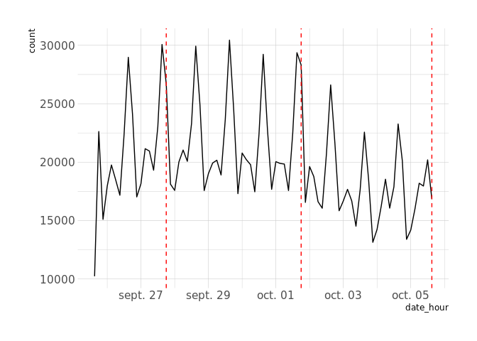
Lets find some anomalies

res <- con %>% 
  wrp_new_gts() %>% 
  wrp_rename("twitter data") %>% 
  wrp_add_value_df(df, tick = "date_hour", value = "count") %>% 
  wrp_bucketize(span = "3 h", bucketizer = "sum") %>% 
  wrp_hybridtest(period = 8, piece = 4, k = 4) %>% 
  wrp_exec()

print(res)
#> [[1]]
#> [[1]][[1]]
#> [1] 3.389256e+14
#> 
#> [[1]][[2]]
#> [1] 3.392712e+14
#> 
#> [[1]][[3]]
#> [1] 3.39606e+14

# Results is a list of abnormal dates in microseconds
res_dbl <- map_dbl(res[[1]], ~ .x / 1e6)

df %>% 
  ggplot(aes(date_hour, count)) +
  geom_line() +
  geom_vline(xintercept = res_dbl, linetype = 2, color = "red") +
  theme_ipsum(base_family = "Verdana")

centreon/warp10r