optimising code for fun and profit
If you’ve ever done some raw-image processing on linux, you’ve probably met dcraw or one of it’s derivatives. You’ve probably also noticed that it is unbearably slow, compared to closed source variants on osx or windows. On a 4 core i7-2600K, 3.4Ghz, developing a 5202x3465 cr2 raw (eos 550d) takes a full 3.3s.
Thankfully dcraw is open source, and being a software geek I felt the need to at least have look. After applying the optimizations documented here, the developing time is reduced to 1.5s.
Without any knowledge to the dcraw code or behaviour (except that the end result is viewable images :) ), we first need to figure out where all that time is spent.
We can get a hint by only using the -v (verbose) option to dcraw.. a lot of time is spent between: “AHD interpolation” and “Converting to sRGB colorspace”. Typically, programmers will write out these messages at the beginning of an algoritm.
First we’ll build with debug enabled (-g to gcc)
on linux we have (at least) two tools for performance analysis: perf and valgrind/callgrind. Let’s try both:
~# perf record -g ./dcraw -w -6 -v test.cr2
~# perf report
+  45.03%  dcraw  dcraw              [.] ahd_interpolate
+  17.60%  dcraw  dcraw              [.] cielab
+   7.46%  dcraw  dcraw              [.] convert_to_rgb
callgrind gives us the same picture
~# valgrind --tool=callgrind ./dcraw -w -6 -v test.cr2
~# kachegrind callgrind.out.*
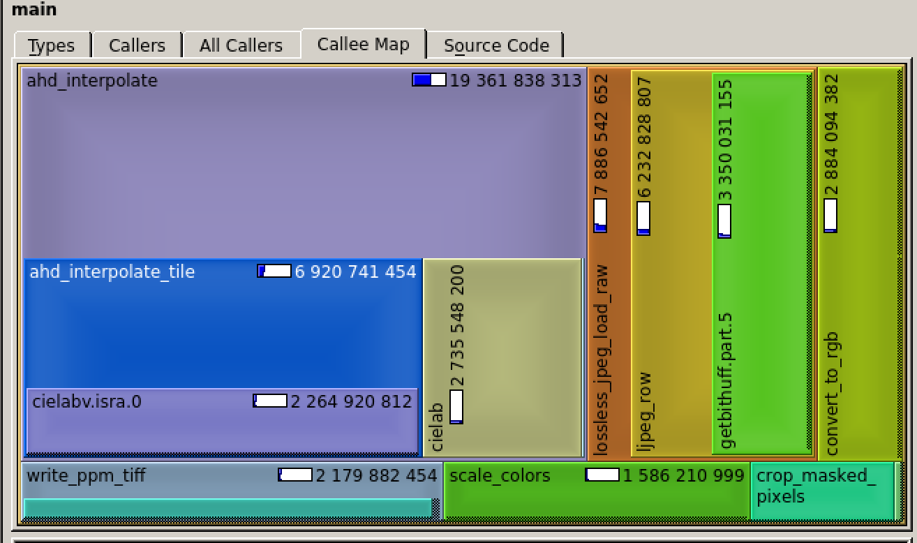
Our suspicion is confirmed. kcachegrind also nicely visualises that cielab is actually part of ahd_interpolate, and that the two together accounts for roughly 50% of the cpu time spent processing test.cr2.
Looking at the ahd_interpolate() function we can see that it is actually composed of several steps: Interpolate green, Interpolate red/blue, Build homogeneity maps and “Combine”.
There are also a couple of other things to note. There seems to be batch processing in “tiles”. If those are independent it should be a nice target for multi-threading. Further there are a lot of nested loops. That’s hardly ever a good sign for performance.
But first, let’s figure out which of the steps take the most time. We’ll do this by simply stop-watch’ing the 4 steps with clock_gettime and accumulate the result. The usual clock source for this task is CLOCK_PROCESS_CPUTIME_ID. This time I opted to use CLOCK_MONOTONIC though, as it’s directly equal to run time (which is what I actually care about).
The result is quite clear:
| stage | runtime |
|---|---|
| green: | .1s |
| red/blue: | .8s |
| “build..”: | .8s |
| combine: | .1s |
| and a total run time, just shy of 2s. |
Modern cpus usually like a couple of properties regarding code and data behaviour.
- Memory access is a speed killer.
- When accessed, memory should ideally be accessed in large linear chunks.
- avoid (unnecessary) branches.
In the “Build homogeneity maps” stage we can find this code:
for (i=0; i < 4; i++)
  if (ldiff[d][i] <= leps && abdiff[d][i] <= abeps)
    homo[d][tr][tc]++;
Since true == 1 on all sane compilers (and this property is actually used elsewhere in dcraw) this can actually be written as
   homo[d][tr][tc]+=
             (ldiff[d][0] <= leps && abdiff[d][0] <= abeps)+
             (ldiff[d][1] <= leps && abdiff[d][1] <= abeps)+
             (ldiff[d][2] <= leps && abdiff[d][2] <= abeps)+
             (ldiff[d][3] <= leps && abdiff[d][3] <= abeps);
That’s removing a for loop (with it’s test and branch) and the if branch. The result is a non neglectable 27% speedup of this stage (0.63s vs 0.8s)
And there is more: there are quite a few uses of the CLIP() macro to keep values within a specific range, specifically within the short int 0 - 0xffff range. The CLIP() macro resolves to two test+branch operations. In the average picture we’ll assume that few of the samples fall outside this range, hence the do nothing case is the dominant one.
overriding branch prediction is slippery slope, but this looks like a perfect opportunity. Using the usual aliases:
 #define likely(x)      __builtin_expect(!!(x), 1)
 #define unlikely(x)    __builtin_expect(!!(x), 0)
we can replace dest=CLIP(val) with:
 dest = val;
 if (unlikely(val<0)) dest=0;
 else if (unlikely(val>0xffff)) dest=0xffff;
That gave me a 19% overall speed gain of ahd_interpolate!
On the other hand, the compiler has features to do these optimisations better than most. We can build a version for profiling, run the code and then feed the profile-info back into the optimisation stage. When collecting the profile it’s important to cover the usual paths. In this case that would probably be to feed it a good sample of different photos. When using profile-guided optimisation, the unlikely() above actually makes the result worse!
The code above also gives us a hint of where we’re going. faster code can also soon become less beautiful, unreadable and unmanageable. (just wait for the SSE variants)
The tiles are actually independent. As such, they are perfect target for threading. We’ll split out the core of ahd_interpolate into a separate ahd_interpolate_tile(top, left, buffer) function that we call call simultaneously from multiple threads.
further, we need a thread_main function for pthread_create, let’s call this ahd_interpolate_worker. It will allocate a thread separate work-buffer and drive the ahd_interpolate_tile for a chunk of tiles. (in this example I’ve split the image vertically in 4 chunks, each thread will do the tiles in it’s chunk)
I’ve also split the cielab function into cielab_init and cielab. This has two gains: The remaining cielab is thread safe (only global reads), and there is an if test less in the interpolate R/B stage.
The remains in ahd_interpolate (_fast) is then basically just to spawn the workers, do one chunk our self and wait for the others to complete.
processing our photo is now done in 1.79s, where 0.5s is spent in ahd_interpolate.
We could call it a day. a ~ 4x speedup (of the algorithm) with 4 threads and almost no code change is really not bad. But we can of course do better.
To better evaluate the gain of the modifications we’ll temporarily revert the threading.
Both interpolate green, and interpolate red/blue run through every pixel. Both also write its resulting pixels to the rgb buffer(s). By combining them we achieve a couple of things:
- the code quickly becomes less readable
- we can arrange the reads in a more optimal way
- we can reduce to one(two) write(s) pr pixel
- since red/blue is depending on the green results, doing these closer together (in time) increases the chance for the green data to be cache hot.
Merging the loops gave ~14% reduction in ahd_interpolate run time
Modern cpu’s like to access memory in chucks of 64 bit words (or even more, SSE vector instructions augments that to 128bit). x86 architecture is somewhat particular in that it allows unaligned access (that is, reading a 8byte word from a non multiple of 8 memory address). Though it is allowed, it does come with a performance penalty, that can be avoided by keeping the data aligned.
the source image (ushort (*image)[4]) fit’s quite nicely in that regard - each pixel occupies 8 bytes.
the temporary buffers are in a worse state: (ushort (*rgb/lab)[3]).
That means almost no pixel position will fall on a 64bit
boundary ( (uintptr_t)(&rgb[d][y][x][c]) & 0x7 almost always != 0 ). We’ll waste a little memory by
redefining them to short(*)[4] and simply ignore the forth element, but it will avoid a lot of unaligned access’
and be faster.
The fastest memory unit to load is almost always the next one. This is because linear access is easily recognised by the pre-fetcher. We’ll therefore give up the tiled design and instead use our chunks from the threading. If memory should be a constraint (the working buffer is now much larger) we could always increase the number of chunks until width * height / chunks == TS * TS
Replacing tiles with chunks gave 1-2% reduction. Not much, but it will also make further changes below easier.
The linear access is really only helpful if we’re actually going to use the next byte. When the cpu fetches data from memory, it will read a whole cache line worth of data, containing the requested address. If we’re only using one, that’s a lot of wasted data transfer. Similarly data is typically transferred from cache to the cpu a word at time (typically that’s 8 bytes). Again, if we could actually use all those bits when they are fetched (or stored) throughput will increase.
The and algorithm stores each pixel twice: the result of vertical and horizontal interpolation. In the original algorithm
this is organised in two separate planes (rgb[d]) TS * TS * 2 * 4 bytes apart. They are always accessed together though.
We can rearrange the layout such that rgb[1][y][x][c] = rgb[0][y][x][c+4]. A bonus is that each rgb pixel is now a full 128 bit SSE register, that can be transferred as one unit.
The above has been a lot of work for minimal gains (going from 1.79s to 1.62s) We shall now harvest some of it.
The vectorisation is terrible work. In dcraw values are 16-bit (ushort), but most of the mathematics require 32-bit precision. I’m targeting sse4 here. sse4 can operate on 4 integers in parallel. The job is then to try and map the steps in the ahd algorithm to do as many 4 parallel operations as possible. Additionally we’ll (half-heartedly) try to minimise memory stalls by keeping operations data-local (e.g.: sum values from line n, then values from line n+1 before summing the results)
As we can see the code is no longer recognisable at all, and without comments it’s really hard to reason about what’s happening. The gain is quite good though: with a single-thread runtime of .9s Reenabling the threads and ahd_interpolate() now accounts for .27s of a total runtime of 1.5s.
Finally I applied vectorisation to a couple of other places (scale_colors in particular)
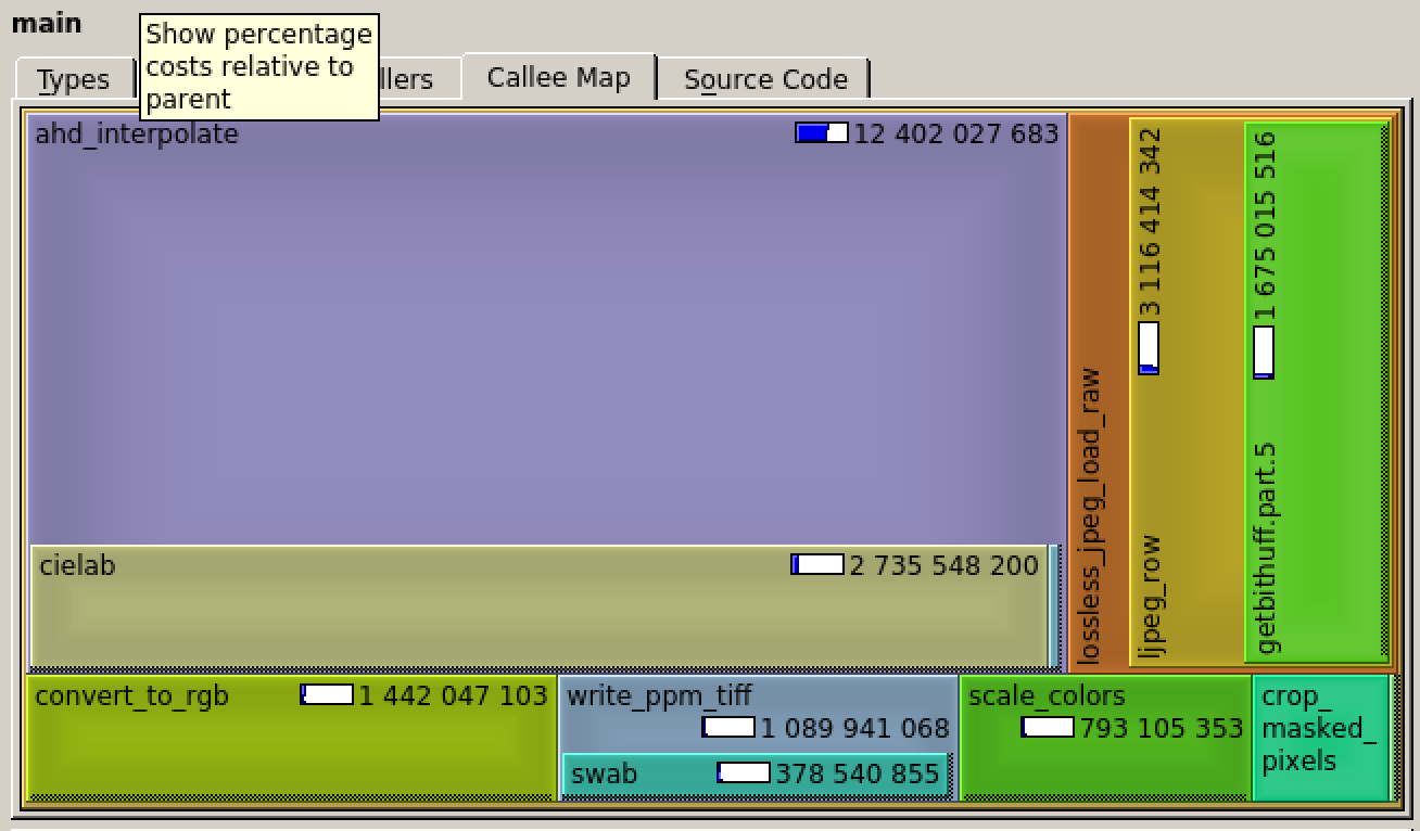
The final cycle distribution looks like this: note that ahd is still a major contributor to cycle count,
but due to threading it spins through them four times as fast!

Jpeg huffman decoding
