cgroza/KU_tutorial_2023

Genotyping using the Human Pangenome Reference

Software requirements

• Please download and install Bandage (https://rrwick.github.io/Bandage/) on your local computer
• The rest of the software will be available in your cloud session:
  • odgi to subset and manipulate genome graphs
  • vg to map reads, count read depth, and call variants
  • bcftools to work with VCF files, call variants
  • samtools to work with BAM files

Long steps in the pipeline

Some steps take a long time that is prohibitive during a workshop. Therefore, long running commands are written to use a small subsample of data that allows you to run the command very fast and understand the tool parameters and output. Later steps then use prepared intermediate files that reside in /data/ to provide the full results.

Data availability

You may download the data at https://doi.org/10.5281/zenodo.10794014.

The Human Pangenome Reference (HPRC)

The Human Pangenome Reference Consortium released the first draft human pangenome reference built from 94 genetically diverse assemblies. This reference uses a graph data structure to represent the known genetic variation at any given locus. Every HPRC genome is a path through the graph and additional genomes are represented as paths that pass through a combination of HPRC genomes.

Genome graphs can be built in various way. The HPRC graph was built from a multiple genome alignment involving 94 assemblies, but graphs can also be built from VCF files. Run vg autoindex to see some options for building graph genomes.

We will open the HPRC graph and inspect some subregions of chromosome 22 with a tool called Bandage. First, we already extracted chromosome 22 from the whole genome graph in the file called hprc-chrom22.odgi. We can use odgi (https://github.com/pangenome/odgi) to ask for specific subgraphs of the human pangenome. For example, this extracts the subgraph of the DGCR6 gene:

Command 1

odgi extract -d 0 -i /data/hprc-chrom22.odgi -c 10 -E -r GRCh38.chr22:18906028-18912088 -o - | odgi view -g -i - > DGCR6.gfa

Key parameters:

• -i input graph
• -r region interval along GRCh38.chr22 path to extract (path:start-end)
• -E extract the subgraph to include nodes and paths from other genomes that touch on GRCh38.chr22. Without this argument, the results will be a simple linear graph without variants
• -c number of surrounding nodes to extract around the specified region. This gives the extracted subgraph a bit more context

Download the file DGCR6.gfa to your own computer by running this on your local UNIX computer. You may ignore -i your_key if you have a username and password:

Command 2

scp -i your_key your_username@52.69.106.213:DGCR6.gfa .

Windows users will have to install PuTTY and use pscp:

Command 3

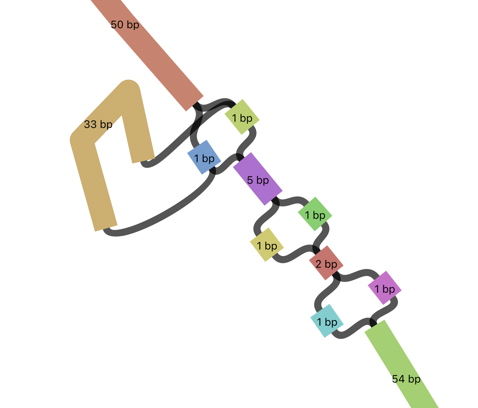
pscp -scp your_username@52.69.106.213:DGCR6.gfa .

Once you have the file, load it in Bandage (File -> Load graph, Draw graph). You should see a long, mostly linear structure. However, you should also see small bubbles along this gene, representing SNVs and indels. In Bandage, use the find node field in the top right of the Bandage window to search for node 270054. You should see a polymorphic region containing a 33 bp indel, and 3 consecutive SNVs within a very short region.

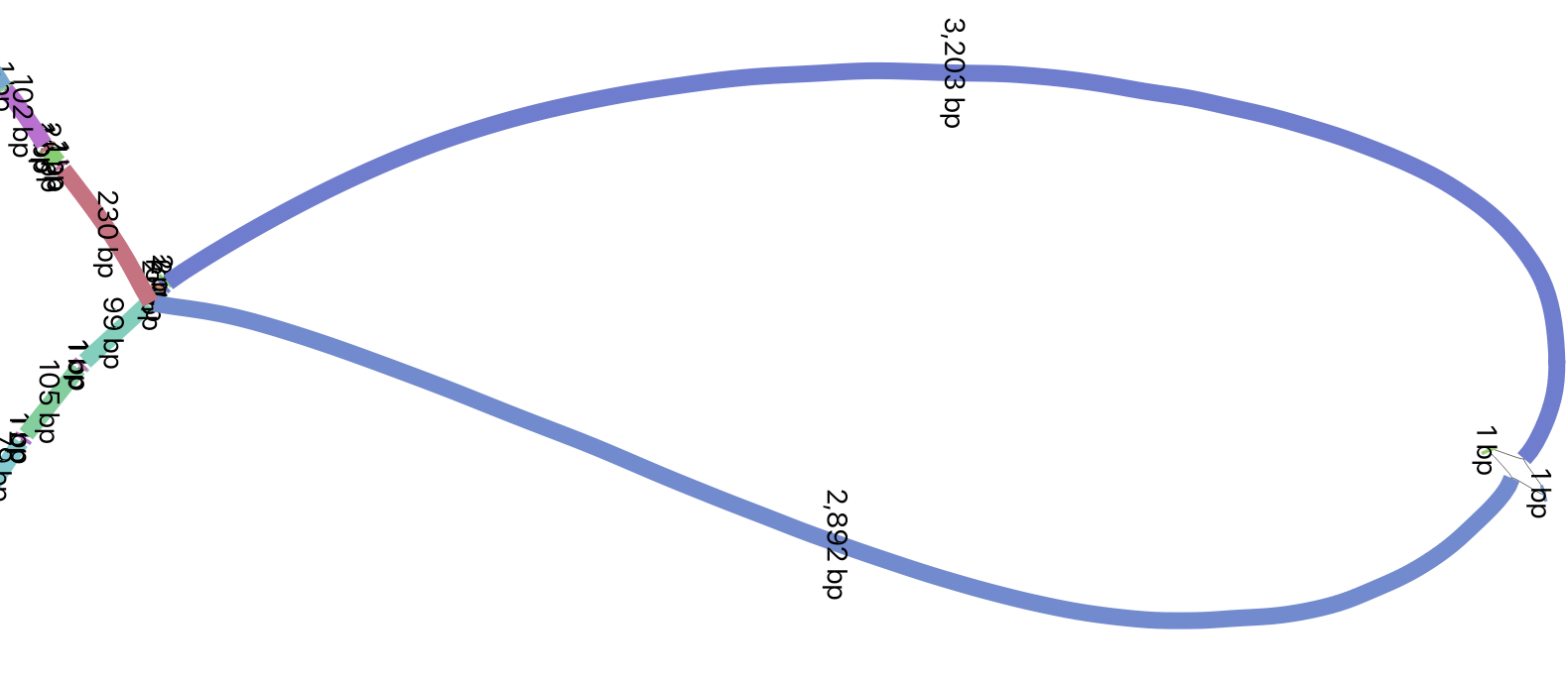
Let’s find a larger structural variant, in this case a 6 kbp LINE1 insertion:

Command 4

odgi extract -d 0 -i /data/hprc-chrom22.odgi -c 100 -E -r GRCh38.chr22:26101249-26121249 -o - | odgi view -g -i - > L1.gfa

Again, download and open the file L1.gfa (just like before, but replace DGCR6.gfa with L1.gfa) in Bandage and find node 438987. You should see something similar to this:

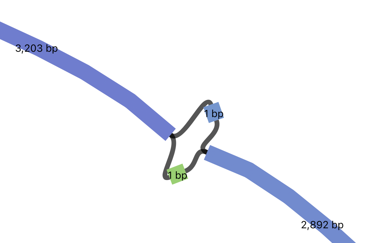
If you zoom in, you should see a small bubble on the L1, representing a SNV nested within the L1 insertion. Note how the graph represents the nested SNP within the LINE1 insertion as a bubble within a bubble:

Mapping whole genome sequencing datasets to the Human Pangenome Reference

We may use the human pangenome reference similarly to how we use GRCh38, to align existing short read data. Let’s align a whole genome sequencing dataset of NA12878 to chr22. We can do this using the graph aligner vg giraffe (https://github.com/vgteam/vg), and the appropriate index files which can be downloaded at https://github.com/human-pangenomics/hpp_pangenome_resources. Here, we align a small sample of reads from chromosome 22 to a graph.

Command 5

vg giraffe -p -i -f /data/NA12878.chr22.sample.fq.gz -Z /data/hprc-chrom22.giraffe.gbz -m /data/hprc-chrom22.min -d /data/hprc-chrom22.dist -o gam  > NA12878.chr22.sample.gam

Key parameters:

• -p show progress
• -i input reads are an interleaved paired-end FASTQ file
• -f input FASTQ file
• -Z input giraffe graph (created with vg autoindex)
• -m minimizer index, a table that lists where the position of k-mers are in the graph
• -d distance index, a table that lets giraffe quickly calculate the minimum distance in bp between any two nodes in the graph
• -o gaf data format for alignments (can be GAM, GAF or others)

At the end of this operation you should see a message similar to this:

Mapped 10044682 reads across 40 threads in 72.2703 seconds with 1.02009 additional single-threaded seconds. Achieved 1469.49 reads per CPU-second (including output)

As you can see, vg giraffe is very fast!

Graph alignments are stored in the GAM or GAF formats

The GAM is a binary format is analogous to the BAM format. It is space efficient but not human readable. GAF is a text file format that is more similar to the SAM file format. While various tools prefer GAF or GAM, vg giraffe allows users to choosing using the -o gaf/gam command line parameter. You can also convert between GAM and GAF using vg convert. You can view a record of the GAF format using:

Command 6

head -n1 /data/NA12878.chr22.sample.gaf

There are many similarities with the BAM/SAM format. For example, there are fields for the read name and its mate, and a mapping quality field. The path field is analogous to the chromosome field but is more complex. As you can see, it is an enumeration of nodes instead of a chromosome and the alignments describe the path in the pangenome on which the read lies. More on the GAF format: https://github.com/lh3/gfatools/blob/master/doc/rGFA.md#the-graph-alignment-format-gaf

Count the read depth on each allele

The aligned whole genome sequencing reads can now be used to genotype variation that is present in the pangenome reference. This approach is particularly useful for genotyping structural variation, which is not accessible to most short read variant callers. To genotype alleles that are present in the graph, we first need to know how many reads align to each allele. We can count this quickly with the following command:

Command 7

vg pack -x /data/hprc-chrom22.giraffe.gbz -g /data/NA12878.chr22.sample.gam -o NA12878.chr22.pack

This creates a pack table that describes how many reads align to each node in the pangenome. Key parameters:

• -x input giraffe graph
• -g input graph alignments from giraffe
• -o output node read depth table

Call variants based on read depth on alleles

We are now ready to call variants using vg call:

Command 8

vg call -r /data/hprc-chrom22.snarls -s NA12878 -k /data/NA12878.chr22.pack /data/hprc-chrom22.giraffe.gbz > NA12878.chr22.hprc.vcf

The output is a VCF file that lists the alleles where NA12878 differs from the GRCh38 path/reference.

Key parameters

• -r index that lets vg quickly find the bubbles in the graph
• -s sample name to be used in VCF
• -k input read depth table from previous step
• input giraffe graph

If you wish to output the genotype of all the alleles, including those that are the same as GRCh38, pass the -a parameter to vg call. This is useful when working with many samples.

Check the number of non-reference variants found

Then, we can quickly summarize the findings with:

Command 9

bcftools stats /data/NA12878.chr22.hprc.vcf | awk -v FS='\t' '$1 == "SN" {print $3,$4}'

The output should reproduce the data in this table:

number of records	37137
number of SNPs	26511
number of MNPs	367
number of indels	10158
number of others	263
number of multiallelic sites	792
number of multiallelic SNP sites	11

Overall, there are 28,636 insertions and 142,417 SNVs in the graph, of which 10,158 indels and 26,511 SNVs are in NA12878. However, NA12878 likely contains many rare SNVs and indels that are not present in the pangenome reference and thus were not called. To recover these, we may still leverage the pangenome reference to remove reference bias and improve our precision and sensitivity. We do so by using these HPRC-corrected alignments with traditional callers such as bcftools, which work on reads aligned to the linear GRCh38 reference.

Projecting alignments from the pangenome to a linear genome

Since GRCh38 is part of the pangenome, it’s relationship to the HPRC genomes is described by the graph. Therefore, any alignment that lies on a bubble can be rewritten as an alignment relative to GRCh38, where the bubble is expressed as an edit. For example, an alignment that matches 23 bp on GRCh38, 64 bp on HG002 and 44 bp on GRCh38 will be projected to GRCh38 as 23M64I44M. Note that there is nothing special about GRCh38, we may project onto any genome in the graph (specified with -p). Project with the following command:

Command 10

vg surject -p GRCh38.chr22 -t 2 -b -x /data/hprc-chrom22.giraffe.gbz /data/NA12878.chr22.sample.gam | samtools sort > NA12878.chr22.hprc.sample.bam

The output file NA12878.chr22.hprc.bam is now a regular BAM file that contains alignments projected onto GRCh38.

Key parameters:

• -p path onto which to project the alignments. Can be any genome that is part of the graph
• -t number of threads to use, more is faster
• -b output BAM
• -x input giraffe graph
• input GAM file to surject to BAM

If you check a record in the BAM file, you will see the path named GRCh38.chr22 in the chromosome field:

Command 11

samtools view NA12878.chr22.hprc.sample.bam | head -n1

This file can be accepted by tools such as DeepVariant or bcftools. Let’s call SNVs and indels with bcftools on HPRC-corrected alignments:

Command 12

bcftools mpileup -Ou -f /data/GRCh38.chr22.fa /data/NA12878.chr22.hprc.sample.bam | bcftools call -mv -Ov -o NA12878.chr22.bcftools.vcf

Let’s summarize the new results just like before:

Command 13

bcftools stats /data/NA12878.chr22.bcftools.vcf | awk -v FS='\t' '$1 == "SN" {print $3,$4}'

Now compare with variants called with bwa mem:

Command 14

bcftools stats /data/NA12878.chr22.bwamem.vcf | awk -v FS='\t' '$1 == "SN" {print $3,$4}'

Indeed we find more SNVs and indels that are unique to NA12878 when we use HPRC-corrected alignments.

Variants	HPRC-corrected	bwa mem	Gain
number of SNPs	65447	67146	-1699
number of indels	14172	10672	3500
number of multiallelic sites	415	349	66
number of multiallelic SNP sites	39	46	-7

At the same time, we can compare to variants called from reads aligned with bwa mem. Indeed, calling variants with HPRC-corrected alignments removes 1699 SNVs (which could be false positives) and gains 3500 indels, which are the most likely to be affected by reference bias.

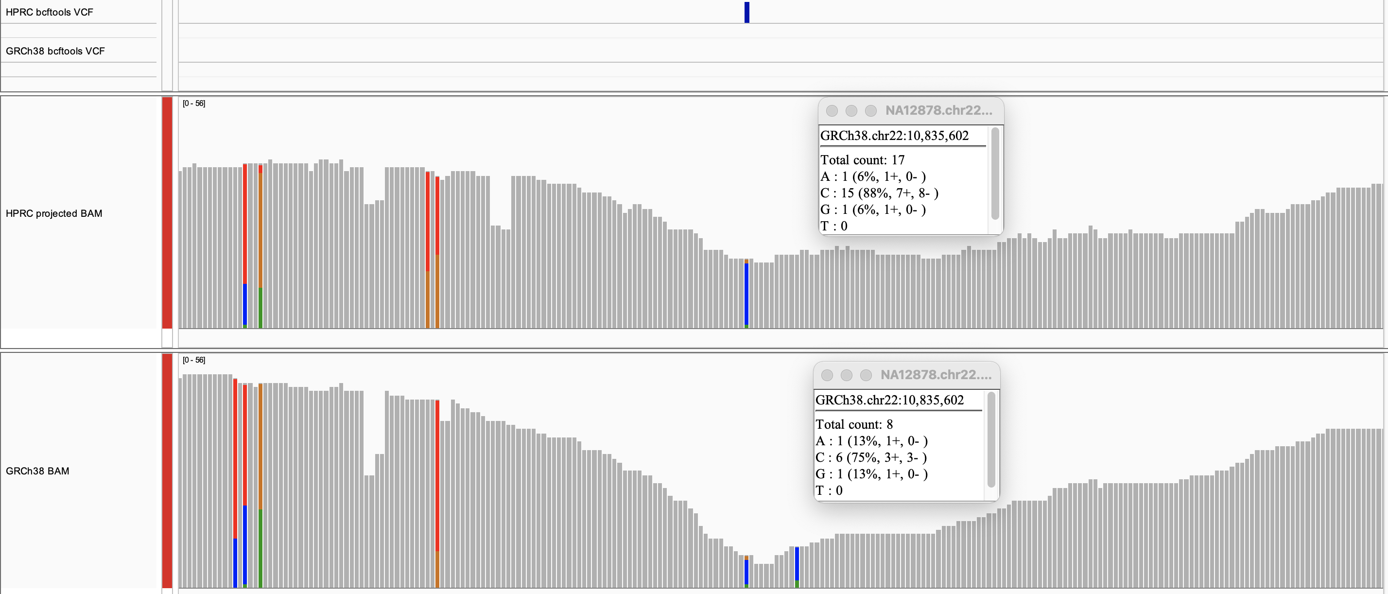
Here we see a SNV that bcftools called with HPRC but missed with GRCh38 alignments in an IGV coverage track:

First, we notice that the read depth on this SNV is slightly higher in HPRC than GRCh38. As shown by the insert tables, HPRC enabled the recovery of 15 reads that support the C SNV, while GRCh38 recovered only 6.

BONUS

The VCF files produced by vg call also indicate which nodes represent the variant.

Command 15

bcftools view -H /data/NA12878.chr22.hprc.vcf | less

The ALT field indicates the source node, the node from which the graph branches out and the sink, the node to which the graph merges again. The source and sink nodes delimit the boundaries of a polymorphic locus. The AT field enumerates the exact path of that variant. As an exercise, pick a variant, subset the graph in this region with odgi, download and visualize it with Bandage by finding the source node of a variant.