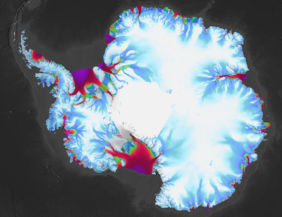
These MATLAB functions are intended to make it easy and efficient to work with ITS_LIVE velocity data.
itslive_mosaic_downloader easily downloads all of the annual mosaics for any specified region.
itslive_data loads ITS_LIVE velocity mosaic data.
itslive_interp interpolates ITS_LIVE velocity mosaic data to specified locations.
itslive_tilefun You probably won't need this function, but it loads multiple years of ITS_LIVE velocity mosaic data in tiles and applies a specified function through time. Tiling is only necessary when memory issues arise when trying to load and process multiple years of ITS_LIVE data all at once. (Requires the Climate Data Toolbox for Matlab.)
itslive_imagesc plots itslive velocity magnitude (speed) data as an imagesc plot. If an AMT polar stereographic map is already open, itslive_imagesc will only load and plot enough data to fill the current map.
itslive_quiver is equivalent to itslive_imagesc, but plots ITS_LIVE velocity data as quiver arrows.
itslive_contour is equivalent to itslive_imagesc, but plots contours instead of scaled color.
itslive_flowline calculates flowlines from itslive velocity mosaics.
itslive_displacement similar to itslive_flowline, but calculates the position of point(s) after a specified time interval. For example, where was a certain grid point 3.5 year ago? Enter its coordinates with a dt value of -3.5 to find out.
itslive_tsplot plots a single grid cell of IT_LIVE velocity observations as a timeseries plot.
Since these functions are currently just for the Antarctic, they rely on Antarctic Mapping Tools for Matlab, so you'll need to get that package if you don't already have it.
If you don't already have the velocity data, download the NetCDF version of the velocity data for your years of interest here. If you only want the mosaic, I recommend the 240 m composite, which provides the error-weighted synthesis of all available data.
After downloading the data, put the NetCDF(s) somewhere Matlab can find them. I personally have a folder called data, and I have a startup.m file in my home directory that contains this line:
addpath(genpath('/Users/cgreene/Documents/MATLAB/data'))
which automatically adds the path to the data folder and all of it subfolders every time I start Matlab.
The ITS_LIVE data and these functions are provided free of charge. All we ask is that you please cite the dataset, and if you're feeling extra generous please do me a kindness and cite my Antarctic Mapping Tools paper too. Wording might be something like, "Velocity data generated using auto-RIFT (Gardner et al., 2018) and provided by the NASA MEaSUREs ITS_LIVE project (Gardner et al., 2019). Analysis was performed with Antarctic Mapping Tools for Matlab (Greene et al., 2017)"
Gardner, A. S., M. A. Fahnestock, and T. A. Scambos, 2019 [update to time of data download]: ITS_LIVE Regional Glacier and Ice Sheet Surface Velocities. Data archived at National Snow and Ice Data Center; doi:10.5067/6II6VW8LLWJ7.
Gardner, A. S., G. Moholdt, T. Scambos, M. Fahnstock, S. Ligtenberg, M. van den Broeke, and J. Nilsson, 2018: Increased West Antarctic and unchanged East Antarctic ice discharge over the last 7 years, Cryosphere, 12(2): 521–547, doi:10.5194/tc-12-521-2018.
Greene, C. A., D. E. Gwyther, and D. D. Blankenship, 2017 “Antarctic Mapping Tools for Matlab.” Computers & Geosciences, (104) 151–157, doi:10.1016/j.cageo.2016.08.003.


