piRF - Prediction Intervals for Random Forests

Chancellor Johnstone and Haozhe Zhang

Introduction

The goal of piRF is to implement multiple state-of-the art random forest prediction interval methodologies in one complete package. Currently, the methods implemented can only be utilized within isolated packages, or the authors have not made a package publicly available. The package itself utilizes the functionality provided by the ranger package. If you utilize this package in any publications, please use the following citation:

Johnstone C, Zhang H (2020). piRF: Prediction Intervals for Random Forests. R package version 0.1.0, https://CRAN.R-project.org/package=piRF.

A BibTeX entry for LaTeX users is

(Manual?){, title = {piRF: Prediction Intervals for Random Forests}, author = {Chancellor Johnstone and Haozhe Zhang}, year = {2020}, note = {R package version 0.1.0}, url = {https://CRAN.R-project.org/package=piRF}, }

Installation

You can install the released version of piRF from CRAN with:

install.packages("piRF")

And the development version from GitHub with:

# install.packages("devtools")
devtools::install_github("chancejohnstone/piRF")

Example

This is a basic example which utilizes the airfoil dataset included with piRF. The dataset comes from UCI Archive. The NASA data set comprises different size NACA 0012 airfoils at various wind tunnel speeds and angles of attack.

The following functions are not exported by piRF but are used for this example.

library(piRF)
## basic example code

data(airfoil)
head(airfoil)
#>   freq AoA length velocity       disp pressure
#> 1  800   0 0.3048     71.3 0.00266337  126.201
#> 2 1000   0 0.3048     71.3 0.00266337  125.201
#> 3 1250   0 0.3048     71.3 0.00266337  125.951
#> 4 1600   0 0.3048     71.3 0.00266337  127.591
#> 5 2000   0 0.3048     71.3 0.00266337  127.461
#> 6 2500   0 0.3048     71.3 0.00266337  125.571

#functions to get average length and average coverage of output
getPILength <- function(x){
#average PI length across each set of predictions
l <- x[,2] - x[,1]
avg_l <- mean(l)
return(avg_l)
}

getCoverage <- function(x, response){
  #output coverage for test data
  coverage <- sum((response >= x[,1]) * (response <= x[,2]))/length(response)
  return(coverage)
}

Prediction intervals are generated for each of the methods implemented using train and test data sets constructed from the airfoil data.

method_vec <- c("quantile", "oob", "bcqrf", "cqrf", "bop", "hdi", "brf")

#generate train and test data
set.seed(2020)
ratio <- .975
nrow <- nrow(airfoil)
n <- floor(nrow*ratio)
samp <- sample(1:nrow, size = n)
train <- airfoil[samp,]
test <- airfoil[-samp,]

#generate fitted models
res <- pirf(pressure ~ . , train_data = train,
            method = method_vec,
            concise= FALSE,
            num_threads = 2,
            alpha = .1)

#generate prediction intervals from fitted models
preds <- predict(res, test_data = test)

In this example, the num_threads option identifies the use of two cores for parallel processing. The default is to use all available cores. The concise option allows for the output of predictions for the test observations.

Below are the coverage rates and average prediction interval lengths using the test dataset. Both are important characteristics of prediction intervals.

#empirical coverage, and average prediction interval length for each method
coverage <- sapply(preds$int, FUN = getCoverage, response = test$pressure)
coverage
#>  quantile       oob     bcqrf      cqrf       bop       hdi       brf 
#> 0.8947368 0.8947368 0.8684211 0.9210526 0.9210526 0.9210526 0.9736842
length <- sapply(preds$int, FUN = getPILength)
length
#>  quantile       oob     bcqrf      cqrf       bop       hdi       brf 
#> 10.233720  7.003722  8.166471 10.958470 12.114255 10.048553  9.004183

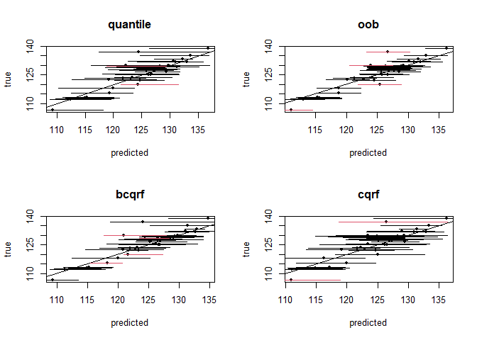
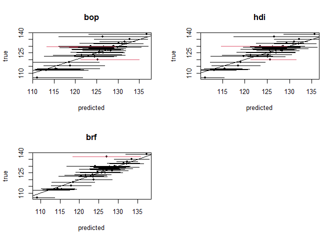
Below are plots of the resulting prediction intervals generated for each method.

#plotting intervals and predictions
par(mfrow = c(2,2))
for(i in 1:length(method_vec)){
  #color based on empirical coverage
  col <- ((test$pressure >= preds$int[[i]][,1]) * (test$pressure <= preds$int[[i]][,2])-1)*(-1)+1
   
  plot(x = preds$preds[[i]], y = test$pressure, pch = 20,
      col = "black", ylab = "true", xlab = "predicted", main = method_vec[i])
  abline(a = 0, b = 1)
  segments(x0 = preds$int[[i]][,1], x1 = preds$int[[i]][,2],
           y1 = test$pressure, y0 = test$pressure, lwd = 1, col = col)
}

If you find any issues with the package, or have suggestions for improvements, please let us know.

References

Breiman, Leo. 2001. “Random Forests.” Machine Learning 45 (1): 5–32. https://link.springer.com/article/10.1023/A:1010933404324.

Ghosal, Indrayudh, and Giles Hooker. 2018. “Boosting Random Forests to Reduce Bias; One-Step Boosted Forest and Its Variance Estimate.” arXiv Preprint. https://arxiv.org/pdf/1803.08000.pdf.

Meinshausen, Nicolai. 2006. “Quantile Regression Forests.” Journal of Machine Learning Research 7 (Jun): 983–99. http://www.jmlr.org/papers/volume7/meinshausen06a/meinshausen06a.pdf.

Romano, Yaniv, Evan Patterson, and Emmanuel Candes. 2019. “Conformalized Quantile Regression.” arXiv Preprint. https://arxiv.org/pdf/1905.03222v1.pdf.

Roy, Marie-Hélène, and Denis Larocque. 2019. “Prediction Intervals with Random Forests.” Statistical Methods in Medical Research. https://doi.org/10.1177/0962280219829885.

Tung, Nguyen Thanh, Joshua Zhexue Huang, Thuy Thi Nguyen, and Imran Khan. 2014. “Bias-Corrected Quantile Regression Forests for High-Dimensional Data.” In 2014 International Conference on Machine Learning and Cybernetics, 1:1–6. IEEE. https://link.springer.com/article/10.1007/s10994-014-5452-1.

Zhang, Haozhe, Joshua Zimmerman, Dan Nettleton, and Daniel J. Nordman. 2019. “Random Forest Prediction Intervals.” The American Statistician, 1–15. https://doi.org/10.1080/00031305.2019.1585288.

Zhu, Lin, Jiaxin Lu, and Yihong Chen. 2019. “HDI-Forest: Highest Density Interval Regression Forest.” arXiv Preprint. https://arxiv.org/pdf/1905.10101.pdf.