This repository contains implementations of the paper
Rapidly Mixing Multiple-try Metropolis Algorithms for Model Selection
Problems
Hyunwoong Chang*, Changwoo J. Lee*, Zhao Tang Luo, Huiyan Sang, and
Quan Zhou,
accepted at NeurIPS 2022,
oral-designated.
We study multiple-try Metropolis (MTM) algorithm (Liu, Liang, and Wong,
2000), which is an extension of the Metropolis-Hastings
(MH) algorithm by selecting the proposed state among multiple trials
according to some weight function
We prove that MTM algorithm with locally balanced weight functions can
achieve a mixing time bound smaller than that of Metropolis-Hastings
(MH) algorithm by a factor of the number of trials
Please see the folder R for the R software codes used in the
simulation studies.
In this demo, we show an illustrative example with Bayesian variable
selection (BVS) problems described in Section 4.1. of the paper.
Consider a high-dimensional linear model with response
Under the sparse statistical model (Hastie, Tibshirani, and Wainwright,
2015) where
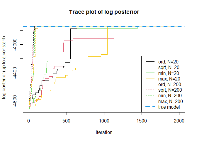
In this brief demo, we investigate the behavior of MTM focusing on implications of the main theorem in our paper:
- As
$N$ increases, mixing time of MTM algorithm becomes smaller by a factor of$N$ . - Using the nondecreasing locally balanced weight function is necessary to establish such result.
First we generate simulated data according to Section 4.1.
## Load libraries, if not installed, install with: install.packages("package name")
library(mgcv) # for Cholesky update
#> Loading required package: nlme
#> This is mgcv 1.8-40. For overview type 'help("mgcv-package")'.
library(matrixStats) # for logsumexp

## data generation
n = 1000; p = 5000; # dimension of design matrix
snr = 4 # signal-to-noise ratio

s = 10; b0 = c(2,-3,2,2,-3,3,-2,3,-2,3); # true model size = 10
beta = c(b0, rep(0, p - s)) * sqrt( log(p)/n ) * snr # true coefficients

set.seed(1)
X = scale(matrix(rnorm(n*p), nrow=n), center = T)
y = X %*% beta + rnorm(n)

# preprocess, take some time
preprocessed = list(
  XtX = crossprod(X),
  Xty = crossprod(X, y),
  yty = crossprod(y)
)
Now we set the initial state of the Markov chain
# initialize gamma (binary vector) s.t. 20 steps needed to reach the true model
gammainit = rep(0,p)
gammainit[sample.int(p-10, size = 10) + 10] = 1

# under hyperparameter settings kappa = 2, g = p^3
kappa = 2; g = p^3;
strue = sum(beta!=0)
SSRtrue = preprocessed$yty - g/(g+1)*t(preprocessed$Xty[1:10])%*%solve(preprocessed$XtX[1:10,1:10],preprocessed$Xty[1:10])
logposttrue = -kappa*strue*log(p) - strue/2*log(1+g) - n/2*log(SSRtrue) # see eq. 13 of the paper
We run the MTM algorithms with
-
$w_{\mathrm{ord}}(y|x) = \pi(y)$ (ordinary, not locally balanced) -
$w_{\mathrm{sqrt}}(y|x) = \sqrt{\pi(y)/\pi(x)}$ (sqrt, locally balanced) -
$w_{\mathrm{min}}(y|x) = \min(\pi(y)/\pi(x),1)$ (min, locally balanced) -
$w_{\mathrm{max}}(y|x) = \max(\pi(y)/\pi(x),1)$ (max, locally balanced)
source("R/bvs_mtm.R") # MTM algorithm for BVS
# ntry = 20
fit_ord_20 = bvs_mtm(y, X, ntry =  20, balancingft = NULL, burn = 0, nmc = 2000,
                       preprocessed = preprocessed, gammainit = gammainit)
#> [1] "balancingft is not provided, using ordinary weight function w(y|x) = p(y)"
#> Run MCMC, initial model size: 10
#> iteration 1000 model size: 10
#> iteration 2000 model size: 10
#> Elapsed time for 2000 MCMC iteration:  0.8634419 secs

fit_sqrt_20 = bvs_mtm(y, X, ntry =  20, balancingft = "sqrt", burn = 0, nmc = 2000,
                      preprocessed = preprocessed, gammainit = gammainit)
#> Run MCMC, initial model size: 10
#> iteration 1000 model size: 9
#> iteration 2000 model size: 10
#> Elapsed time for 2000 MCMC iteration:  0.64868 secs

fit_min_20 = bvs_mtm(y, X, ntry =  20, balancingft = "min", burn = 0, nmc = 2000,
                     preprocessed = preprocessed, gammainit = gammainit)
#> Run MCMC, initial model size: 10
#> iteration 1000 model size: 11
#> iteration 2000 model size: 10
#> Elapsed time for 2000 MCMC iteration:  0.710078 secs

fit_max_20 = bvs_mtm(y, X, ntry =  20, balancingft = "max", burn = 0, nmc = 2000,
                     preprocessed = preprocessed, gammainit = gammainit)
#> Run MCMC, initial model size: 10
#> iteration 1000 model size: 9
#> iteration 2000 model size: 10
#> Elapsed time for 2000 MCMC iteration:  0.690932 secs

# ntry = 200
fit_ord_200 = bvs_mtm(y, X, ntry =  200, balancingft = NULL, burn = 0, nmc = 2000,
                     preprocessed = preprocessed, gammainit = gammainit)
#> [1] "balancingft is not provided, using ordinary weight function w(y|x) = p(y)"
#> Run MCMC, initial model size: 10
#> iteration 1000 model size: 10
#> iteration 2000 model size: 10
#> Elapsed time for 2000 MCMC iteration:  1.384647 secs

fit_sqrt_200 = bvs_mtm(y, X, ntry =  200, balancingft = "sqrt", burn = 0, nmc = 2000,
                      preprocessed = preprocessed, gammainit = gammainit)
#> Run MCMC, initial model size: 10
#> iteration 1000 model size: 10
#> iteration 2000 model size: 10
#> Elapsed time for 2000 MCMC iteration:  1.293503 secs

fit_min_200 = bvs_mtm(y, X, ntry =  200, balancingft = "min", burn = 0, nmc = 2000,
                     preprocessed = preprocessed, gammainit = gammainit)
#> Run MCMC, initial model size: 10
#> iteration 1000 model size: 10
#> iteration 2000 model size: 10
#> Elapsed time for 2000 MCMC iteration:  1.309706 secs

fit_max_200 = bvs_mtm(y, X, ntry =  200, balancingft = "max", burn = 0, nmc = 2000,
                     preprocessed = preprocessed, gammainit = gammainit)
#> Run MCMC, initial model size: 10
#> iteration 1000 model size: 10
#> iteration 2000 model size: 10
#> Elapsed time for 2000 MCMC iteration:  1.344248 secs

# plot
plot(fit_ord_20$logpostout, type="l", main = "Trace plot of log posterior", xlab = "iteration", ylab="log posterior (up to a constant)")
lines(fit_sqrt_20$logpostout, col = 2)
lines(fit_min_20$logpostout, col = 3)
lines(fit_max_20$logpostout, col = 7)
lines(fit_ord_200$logpostout, col = 1, lty = 2)
lines(fit_sqrt_200$logpostout, col = 2, lty = 2)
lines(fit_min_200$logpostout, col = 3, lty = 2)
lines(fit_max_200$logpostout, col = 7, lty = 2)
abline(h = logposttrue, col = 4, lty = 2, lwd =3)
legend("bottomright",lty = c(1,1,1,1,2,2,2,2,2),
       col = c(1,2,3,7,1,2,3,7,4),lwd = c(1,1,1,1,1,1,1,1,3),
       legend = c("ord, N=20","sqrt, N=20","min, N=20","max, N=20",
                  "ord, N=200","sqrt, N=200","min, N=200","max, N=200",
                  "true model"))
We can check that MTM with
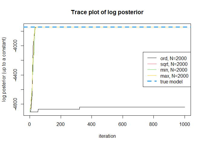
In above example when
### ntry = 2000
fit_ord_2000 = bvs_mtm(y, X, ntry =  2000, balancingft = NULL, burn = 0, nmc = 1000,
                     preprocessed = preprocessed, gammainit = gammainit)
#> [1] "balancingft is not provided, using ordinary weight function w(y|x) = p(y)"
#> Run MCMC, initial model size: 10
#> iteration 1000 model size: 10
#> Elapsed time for 1000 MCMC iteration:  4.016815 secs

fit_sqrt_2000 = bvs_mtm(y, X, ntry =  2000, balancingft = "sqrt", burn = 0, nmc = 1000,
                      preprocessed = preprocessed, gammainit = gammainit)
#> Run MCMC, initial model size: 10
#> iteration 1000 model size: 10
#> Elapsed time for 1000 MCMC iteration:  3.224952 secs

fit_min_2000 = bvs_mtm(y, X, ntry =  2000, balancingft = "min", burn = 0, nmc = 1000,
                        preprocessed = preprocessed, gammainit = gammainit)
#> Run MCMC, initial model size: 10
#> iteration 1000 model size: 10
#> Elapsed time for 1000 MCMC iteration:  3.184143 secs

fit_max_2000 = bvs_mtm(y, X, ntry =  2000, balancingft = "max", burn = 0, nmc = 1000,
                        preprocessed = preprocessed, gammainit = gammainit)
#> Run MCMC, initial model size: 10
#> iteration 1000 model size: 10
#> Elapsed time for 1000 MCMC iteration:  2.977435 secs

plot(fit_sqrt_2000$logpostout, type = "l", main = "Trace plot of log posterior", xlab = "iteration", ylab="log posterior (up to a constant)")
lines(fit_ord_2000$logpostout, col = 1)
lines(fit_min_2000$logpostout, col = 3)
lines(fit_max_2000$logpostout, col = 7)
abline(h = logposttrue, col = 4, lty = 2, lwd =3)
legend("right", lty = c(1,1,1,1,2), col = c(1,2,3,7,4),lwd = c(1,1,1,1,3),
       legend = c("ord, N=2000","sqrt, N=2000","min, N=2000","max, N=2000",
                  "true model"))
We can clearly see that MTM with
Chang, H., Lee, C. J., Luo, Z. T., Sang, H., & Zhou, Q. (2022). Rapidly Mixing Multiple-try Metropolis Algorithms for Model Selection Problems. Advances in Neural Information Processing Systems 35 (NeurIPS), just-accepted.
Hastie, T., Tibshirani, R., & Wainwright, M. (2015). Statistical learning with sparsity. Monographs on statistics and applied probability, 143, 143.
Liu, J. S., Liang, F., & Wong, W. H. (2000). The multiple-try method and local optimization in Metropolis sampling. Journal of the American Statistical Association, 95(449), 121-134.

