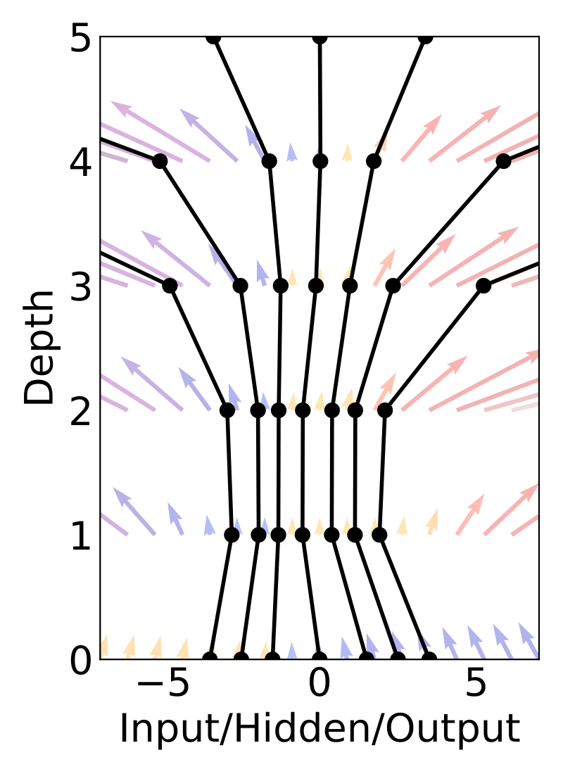
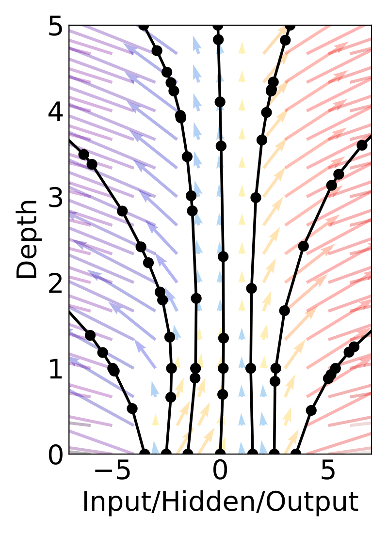
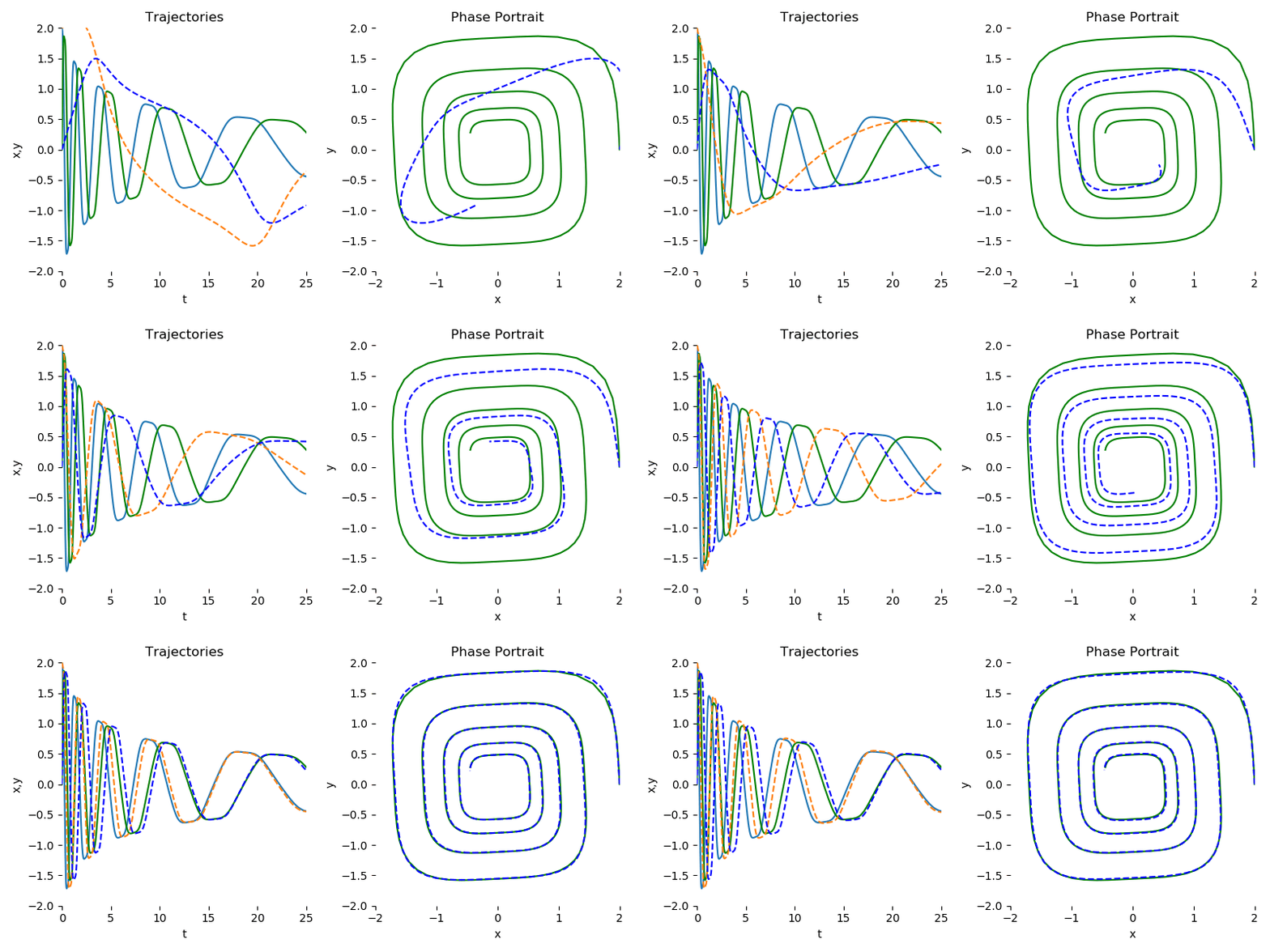
PyTorch Implementation of Differentiable ODE Solvers

This library provides ordinary differential equation (ODE) solvers implemented in PyTorch. Backpropagation through all solvers is supported using the adjoint method. For usage of ODE solvers in deep learning applications, see [1].

As the solvers are implemented in PyTorch, algorithms in this repository are fully supported to run on the GPU.

Installation

pip install torchdiffeq

Examples

Examples are placed in the examples directory.

We encourage those who are interested in using this library to take a look at examples/ode_demo.py for understanding how to use torchdiffeq to fit a simple spiral ODE.

Basic usage

This library provides one main interface odeint which contains general-purpose algorithms for solving initial value problems (IVP), with gradients implemented for all main arguments. An initial value problem consists of an ODE and an initial value,

dy/dt = f(t, y)    y(t_0) = y_0.

The goal of an ODE solver is to find a continuous trajectory satisfying the ODE that passes through the initial condition.

To solve an IVP using the default solver:

from torchdiffeq import odeint

odeint(func, y0, t)

where func is any callable implementing the ordinary differential equation f(t, x), y0 is an any-D Tensor representing the initial values, and t is a 1-D Tensor containing the evaluation points. The initial time is taken to be t[0].

Backpropagation through odeint goes through the internals of the solver. Note that this is not numerically stable for all solvers (but should probably be fine with the default dopri5 method). Instead, we encourage the use of the adjoint method explained in [1], which will allow solving with as many steps as necessary due to O(1) memory usage.

To use the adjoint method:

from torchdiffeq import odeint_adjoint as odeint

odeint(func, y0, t)

odeint_adjoint simply wraps around odeint, but will use only O(1) memory in exchange for solving an adjoint ODE in the backward call.

The biggest gotcha is that func must be a nn.Module when using the adjoint method. This is used to collect parameters of the differential equation.

Keyword Arguments

rtol Relative tolerance.
atol Absolute tolerance.
method One of the solvers listed below.
options A dictionary of solver-specific options, see the further documentation.

List of ODE Solvers:

Adaptive-step:

dopri8 Runge-Kutta 7(8) of Dormand-Prince-Shampine
dopri5 Runge-Kutta 4(5) of Dormand-Prince [default].
bosh3 Runge-Kutta 2(3) of Bogacki-Shampine
adaptive_heun Runge-Kutta 1(2)

Fixed-step:

euler Euler method.
midpoint Midpoint method.
rk4 Fourth-order Runge-Kutta with 3/8 rule.
explicit_adams Explicit Adams-Bashforth.
implicit_adams Implicit Adams-Bashforth-Moulton.

For most problems, good choices are the default dopri5, or to use rk4 with options=dict(step_size=...) set appropriately small. Adjusting the tolerances (adaptive solvers) or step size (fixed solvers), will allow for trade-offs between speed and accuracy.

Frequently Asked Questions

Take a look at our FAQ for frequently asked questions.

Further documentation

For details of the adjoint-specific and solver-specific options, check out the further documentation.

References

[1] Ricky T. Q. Chen, Yulia Rubanova, Jesse Bettencourt, David Duvenaud. "Neural Ordinary Differential Equations." Advances in Neural Information Processing Systems. 2018. [arxiv]

If you found this library useful in your research, please consider citing

@article{chen2018neural,
  title={Neural Ordinary Differential Equations},
  author={Chen, Ricky T. Q. and Rubanova, Yulia and Bettencourt, Jesse and Duvenaud, David},
  journal={Advances in Neural Information Processing Systems},
  year={2018}
}

charlie-chaoscat/torchdiffeq