Network flow optimization of California's water supply system. Requires: NumPy/SciPy/Pandas (all available in the Anaconda Distribution, and Pyomo.
Recommended command-line method to install Pyomo (only tested with Python 3.4):
conda install pyomo pyomo.extras glpk --channel cachemeorgThis will install the GLPK solver. Pyomo can also connect to other solvers, including CBC and CPLEX, and Gurobi. Installation of these solvers is not covered here. UC Davis: these are installed on HPC1 in /group/hermangrp/.
- Clone repository
git clone https://github.com/ucd-cws/calvin
- Get network data (links). CSV file with column headers:
i,j,k,cost,amplitude,lower_bound,upper_bound
Where i,j,k are the source node, destination node, and piecewise index for the network problem. Each row is a link. The California network data files are too large to host on Github; they can be downloaded here:
- 1-year example (WY 1922, 1 CSV file, 400 KB)
- 82-year perfect foresight (1 CSV file, 27 MB)
- Annual, limited foresight (ZIP of 82 CSV files, 31 MB)
To export other subsets of the network (in space or time), see the advanced readme for data export from HOBBES.
-
Create a Python script to import the network data and run the optimization. It is recommended to first run in "debug mode" to identify and remove infeasibilities in the network.
# main-example.py
from calvin import *

calvin = CALVIN('linksWY1922.csv')

# run in debug mode. reduces LB constraints.
calvin.create_pyomo_model(debug_mode=True, debug_cost=2e10)
calvin.solve_pyomo_model(solver='glpk', nproc=1, debug_mode=True)

# run without debug mode (should be feasible)
calvin.create_pyomo_model(debug_mode=False)
calvin.solve_pyomo_model(solver='glpk', nproc=1, debug_mode=False)

postprocess(calvin.df, calvin.model, resultdir='example-results')
# creates output CSV files in the directory specified
Running
python main-example.pyon the command line will show:Creating Pyomo Model (debug=True) -----Solving Pyomo Model (debug=True) Finished. Fixing debug flows... SR_ML.1922-09-30_FINAL UB raised by 8.28 (0.28%) -----Solving Pyomo Model (debug=True) Finished. Fixing debug flows... All debug flows eliminated (iter=2, vol=8.28) Creating Pyomo Model (debug=False) -----Solving Pyomo Model (debug=False) Optimal Solution Found (debug=False).
-
The folder
example-resultswill contain 8 CSV files. All are timeseries data, each row is 1 month. Recommended to read these intopandasfor further analysis:df = pd.read_csv(filename, index_col=0, parse_dates=True).flow.csv(flows on links, TAF/month, columns are link names)storage.csv(end-of-month surface and GW storage, TAF)dual_lower.csv(dual values on lower bound constraints)dual_upper.csv(dual values on upper bound constraints)dual_node.csv(dual values on mass balance constraints)shortage_volume.csv(water supply shortage, relative to demand, on selected links and aggregated regions)shortage_cost.csv(cost of water supply shortage, for selected links and aggregated regions)evaporation.csv(TAF/month)
Several of the solvers available through Pyomo support shared-memory parallelization. (Importantly GLPK is one exception that does not support parallelization). To take advantage of this, change the script above to include:
calvin.solve_pyomo_model(solver='cplex', nproc=32, debug_mode=True)
# do the same again for the non-debug mode run
Several job scripts are included to support running on a SLURM cluster such as HPC1 at UC Davis. These will need to be customized for each system.
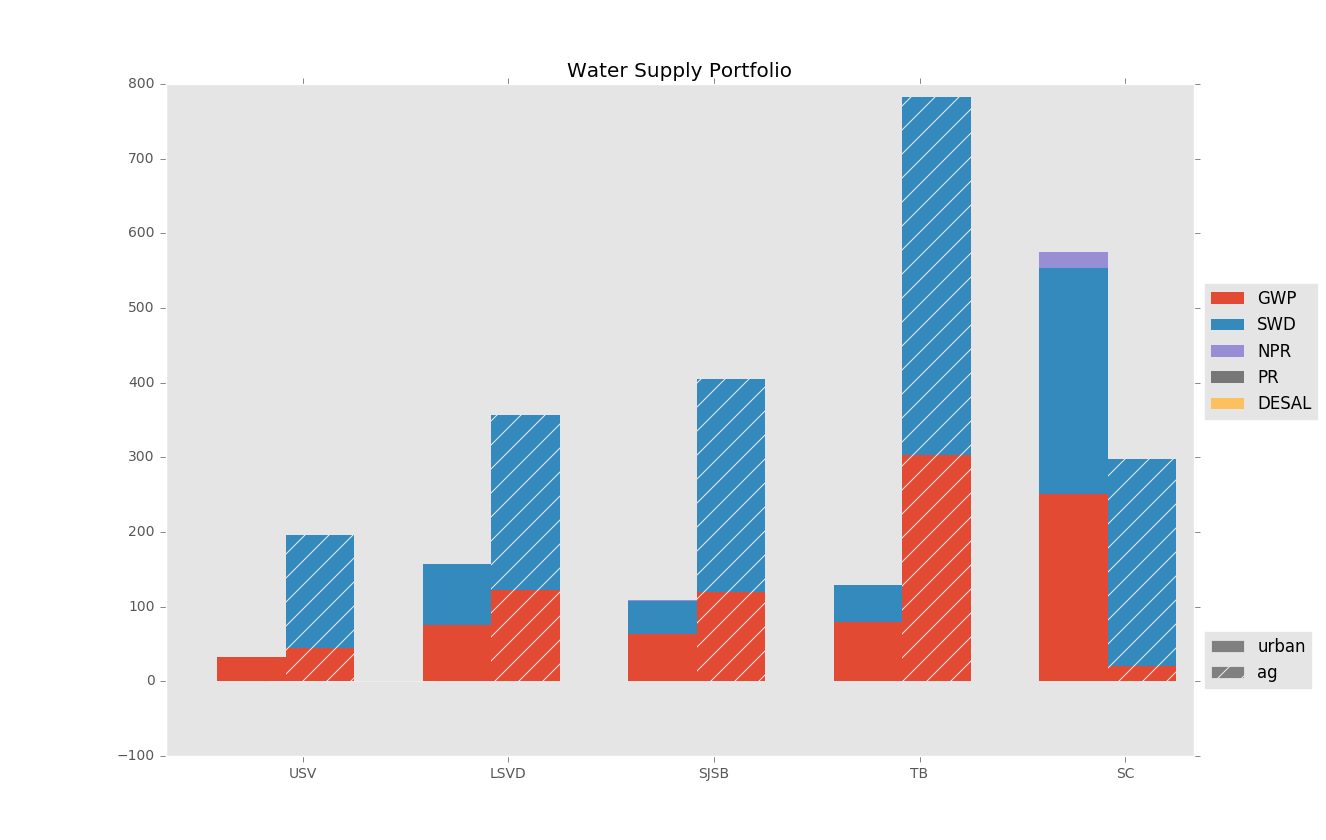
In general, plotting results is left to the user. A few useful plot types will be included in calvin/plots.py. One example is the supply portfolio stacked bar chart, which plots the sum of flows by each region, supply type, and urban/agricultural link type:
The Documentation describes the model in more detail. This refers to an earlier version of the model using Pyomo's AbstractModel type, but the setup is mostly the same in the current ConcreteModel. There is also detailed Pyomo documentation.
