Exploring the concept of knowledge informed machine learning with the use of a Weibull-based loss function. Used to predict remaining useful life (RUL) on the IMS and PRONOSTIA (also called FEMTO) bearing data sets.
Knowledge informed machine learning is used on the IMS and PRONOSTIA bearing data sets for remaining useful life (RUL) prediction. The knowledge is integrated into a neural network through a novel Weibull-based loss function. A thorough statistical analysis of the Weibull-based loss function is conducted, demonstrating the effectiveness of the method on the PRONOSTIA data set. However, the Weibull-based loss function is less effective on the IMS data set.
The experiment is detailed in the Journal of Prognostics and Health Management, with an extensive discussion on the results, shortcomings, and benefits analysis. The paper also gives an overview of knowledge informed machine learning as it applies to prognostics and health management (PHM).
You can reproduce the work, and all figures, by following the instructions in the Setup section. Even easier: run the Colab notebook!
If you have any questions, leave a comment in the discussion, or email me (18tcvh@queensu.ca).
Feel free to cite my research if you use it in any academic research.
@article{von2022knowledge,
  title={Knowledge Informed Machine Learning using a Weibull-based Loss Function},
  author={von Hahn, Tim and Mechefske, Chris K},
  journal={Journal of Prognostics and Health Management},
  volume={2},
  number={1},
  pages={9--44},
  year={2022}
}
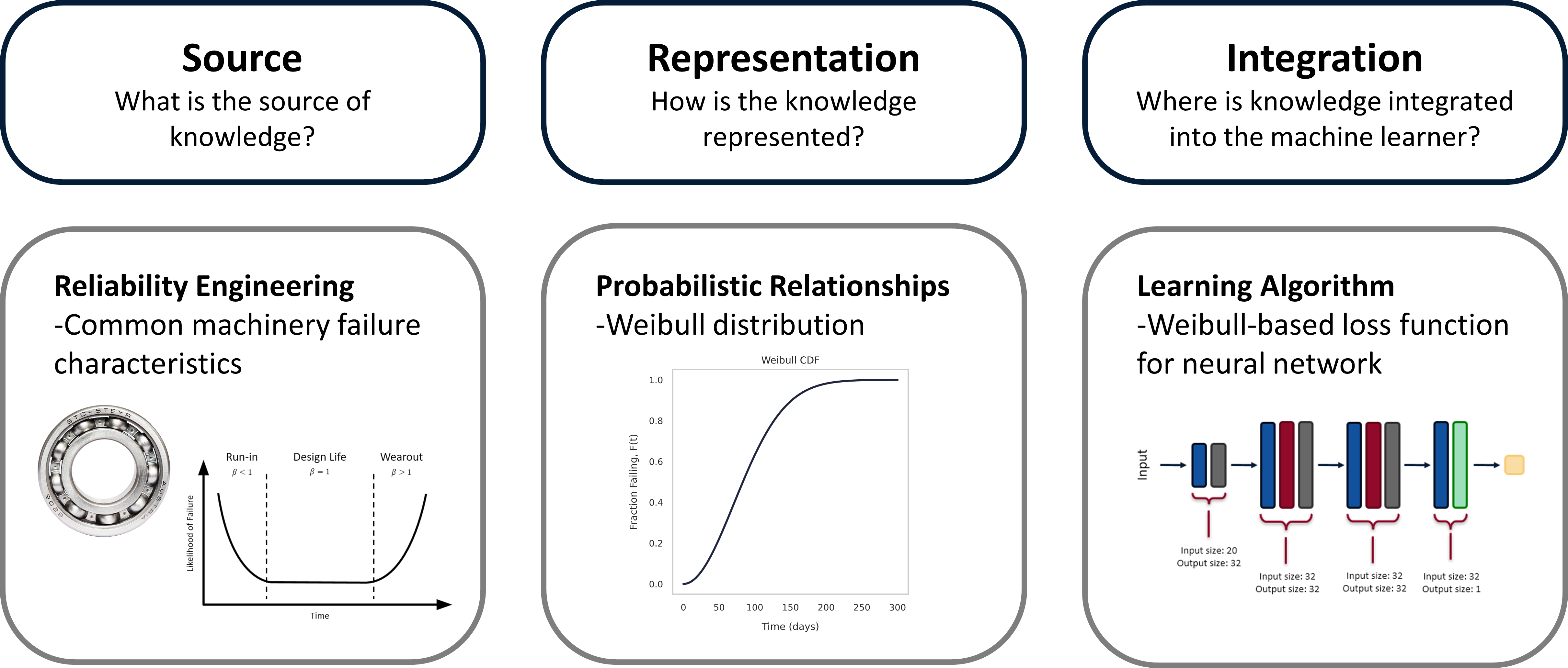
In this work, we use the definition of knowledge informed machine learning from von Rueden et al. (their excellent paper is here). Here's the general taxonomy of our knowledge informed machine learning experiment:
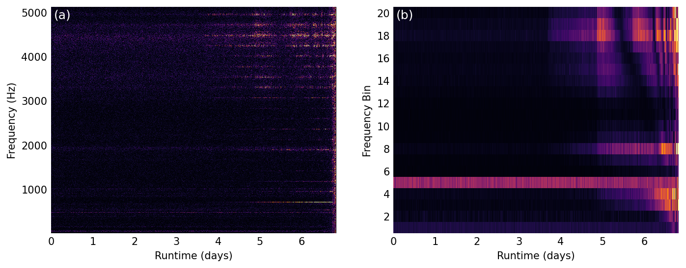
Bearing vibration data (from the frequency domain) was used as input to feed-forward neural networks. The below figure demonstrates the data as a spectrogram (a) and the spectrogram after "binning" (b). The binned data was used as input.
A large hyper-parameter search was conducted on neural networks. Nine different Weibull-based loss functions were tested on each unique network.
The below chart is a qualitative method of showing the effectiveness of the Weibull-based loss functions on the two data sets.
We also conducted a statistical analysis of the results, as shown below.
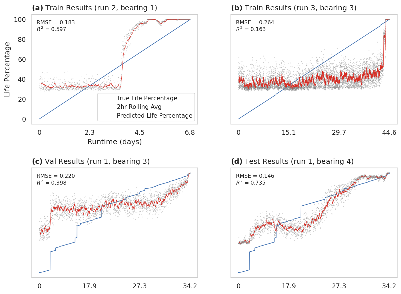
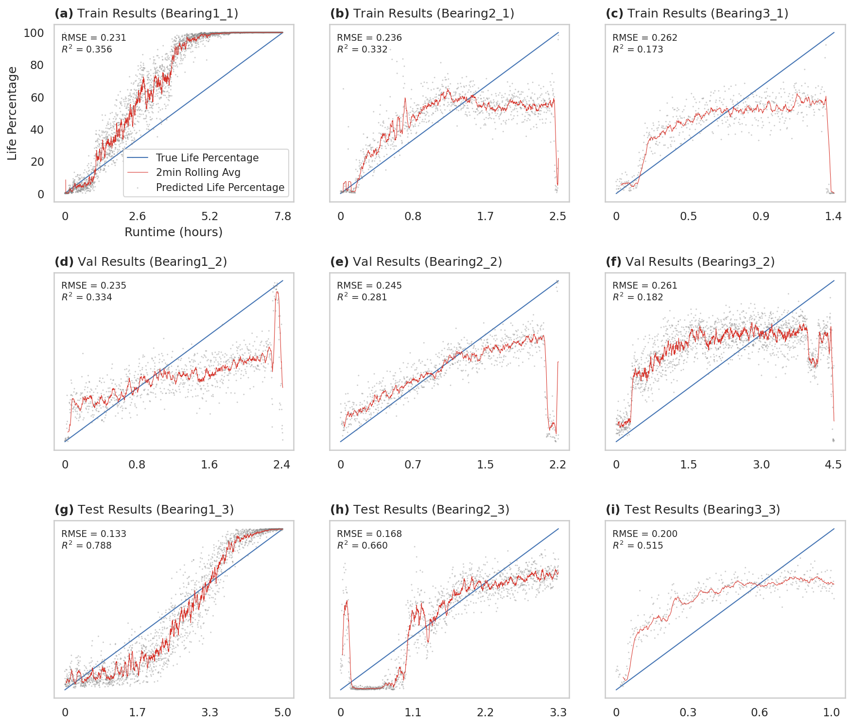
The top performing models' RUL trends are shown below, for both the IMS and PRONOSTIA data sets.
Tested in linux (MacOS should also work). If you run windows you'll have to do much of the environment setup and data download/preprocessing manually.
To reproduce results:
-
Clone this repo -
clone https://github.com/tvhahn/weibull-knowledge-informed-ml.git -
Create virtual environment. Assumes that Conda is installed.
- Linux/MacOS: use command from the Makefile in the root directory -
make create_environment - Windows: from root directory -
conda env create -f envweibull.yml - HPC:
make create_environmentwill detect HPC environment and automatically create environment frommake_hpc_venv.sh. Tested on Compute Canada. Modifymake_hpc_venv.shfor your own HPC cluster.
- Linux/MacOS: use command from the Makefile in the root directory -
-
Download raw data.
-
Extract raw data.
- Linux/MacOS: use
make extract. Will automatically extract to appropriatedata/rawdirectory. - Windows: Manually extract data. See the Project Organization section for folder structure.
- HPC: use
make download. Will automatically detect HPC environment. Again, modify for your HPC cluster.
- Linux/MacOS: use
-
Ensure virtual environment is activated.
conda activate weibullorsource ~/weibull/bin/activate -
From root directory of
weibull-knowledge-informed-ml, runpip install -e .-- this will give the python scripts access to thesrcfolders. -
Train!
-
Linux/MacOS: use
make train_imsormake train_femto. Note: set constants in the makefile for changing random search parameters. Currently set as default.-
Windows: run manually by calling the script -
python train_imsorpython train_femtowith the appropriate arguments. For example:src/models/train_models.py --data_set femto --path_data your_data_path --proj_dir your_project_directory_path -
HPC: use
make train_imsormake train_femto. The HPC environment should be automatically detected. A SLURM script will be run for a batch job.- Modify the
train_modify_ims_hpc.shortrain_model_femto_hpc.shin thesrc/modelsdirectory to meet the needs of your HPC cluster. This should work on Compute Canada out of the box.
- Modify the
-
-
-
Filter out the poorly performing models and collate the results. This will create several results files in the
models/finalfolder.- Linux/MacOS: use
make summarize_ims_modelsormake summarize_femto_models. (note: set filter boundaries insummarize_model_results.py. Will eventually modify for use with Argparse...) - Windows: run manually by calling the script.
- HPC: use
make summarize_ims_modelsormake summarize_femto_models. Again, change filter requirements in thesummarize_model_results.pyscript.
- Linux/MacOS: use
-
Make the figures of the data and results.
- Linux/MacOS: use
make figures_dataandmake figures_results. Figures will be generated and placed in thereports/figuresfolder. - Windows: run manually by calling the script.
- HPC: use
make figures_dataandmake figures_results
- Linux/MacOS: use
├── LICENSE
├── Makefile           <- Makefile with commands to reproduce work, lik `make data` or `make train_ims`
├── README.md          <- The top-level README.
├── data
│   ├── interim        <- Intermediate data that has been transformed.
│   ├── processed      <- The final, canonical data sets for modeling.
│   └── raw            <- The original, immutable data dump. Downloaded from the NASA Prognostic repository.
│
├── docs               <- A default Sphinx project; see sphinx-doc.org for details (nothing in here yet)
│
├── models             <- Trained models, model predictions, and model summaries
│   ├── interim        <- Intermediate models that have not analyzed. Output from the random search.
│   ├── final          <- Final models that have been filtered and summarized. Several outpu csv files as well.
│
├── notebooks          <- Jupyter notebooks used for data exploration and analysis. Of varying quality.
│   ├── scratch        <- Scratch notebooks for quick experimentation.
│
├── references         <- Data dictionaries, manuals, and all other explanatory materials (empty).
│
├── reports            <- Generated analysis as HTML, PDF, LaTeX, etc.
│   └── figures        <- Generated graphics and figures to be used in reporting
│
├── requirements.txt   <- The requirements file for reproducing the analysis environment, e.g.
│                         generated with `pip freeze > requirements.txt`
│
├── envweibull.yml    <- The Conda environment file for reproducing the analysis environment
│                        recommend using Conda).
│
├── make_hpc_venv.sh  <- Bash script to create the HPC venv. Setup for my Compute Canada cluster.
│                        Modify to suit your own HPC cluster.
│
├── setup.py           <- makes project pip installable (pip install -e .) so src can be imported
├── src                <- Source code for use in this project.
│   ├── __init__.py    <- Makes src a Python module
│   │
│   ├── data           <- Scripts to download or generate data
│   │   └── make_dataset.py
│   │
│   ├── features       <- Scripts to turn raw data into features for modeling
│   │   └── build_features.py
│   │
│   ├── models         <- Scripts to train models
│   │   └── predict_model.py
│   │
│   └── visualization  <- Scripts to create figures of the data, results, and training progress
│       ├── visualize_data.py
│       ├── visualize_results.py
│       └── visualize_training.py
As noted in the paper, the best thing would be to test out Weibull-based loss functions on large, and real-world, industrial datasets. Suitable applications may include large fleets of pumps or gas turbines.


