All examples to run VDAT and scripts to generate plots are located in <path_to_VDATN3multi>/src/example/. The following code snippets may be outdated, please refer to the lastest version of the code to find the correct usage.
To start with, include the vdat.jl. The following code assumes current path is <path_to_VDATN3multi>/src/example/
To start with, let's solve the one band Hubbard on a d=\infty Bethe lattice. There are two modes to work with, the fixed density mode and the free density mode. In fixed density mode, one can specify the density for each spin orbital, and VDAT automatically constrains the variational parameters to satify the given densities. For example, we start with half-filling case, which exhibits the metal-insulator transition at some critical U. To perform the VDAT calculation, we need to build an instance of Model, which can be created with create_model.
VDATN3multi.jl/src/example/example_one_band_half.jl
Lines 5 to 15 in 8afb25f
This is the typical way how we construct the model, so we examine the above code line-by-line. N_spin_oribital_ specifies the number of spin-oribtals of the model. We normally label these spin orbitals from 1 to N_spin_orbital_. The variable symmetry_ defines the symmetry of the model, which has the form like [symmetry_group1,symmetry_group2,..,symmetry_groupN] where symmetry_groupi=[spin_orb_1,spin_orb_2,..spin_orb_M]. Each entry of symmetry_ is array of the index of spin-orbitals which have permutation symmetry within themselves. The variable n_target_ has the form [n_group1, n_group2,..,n_groupN], which must has the same length as as symmetry_, and specify the density per spin orbital within each symmetry group. Correspondingly, for each symmetry group, we can also specify the density of states D(e). To parametrize D(e), one can sample the energies from D(e) and store them ascendingly in a file, which can be loaded by gene_spline_band. Finally, the two body interaction is specified by the variable interaction_ which is a array of tuple and has the form like [(i,j,Uij)...], where i,j are the index of two different spin-orbitals and each tuple corresponds a interaction like Uij * ni * nj. Similarly, the one body interaction is specified by the chemical_potential_, which has the form like [(i,mui)...], and each tuple corresponds a term like -mui * ni.
Once we create the model, we can use get_para and set_para to view and write the variational parameters. Furthermore, function compute will evaluation the total energy and other observables for the given variational parameters. All observables can be read from model.obs, or using @get_obs macro.
VDATN3multi.jl/src/example/example_one_band_half.jl
Lines 18 to 36 in 8afb25f
While we focus for VDAT N=3, we also implement N=2 (equivalent to the well-known Gutzwiller approximation) using the same interface. One can simply set N_time_step=2 when creating the model, and remaining part is almost identical (The exception is that one get fewer observables in model.obs in N=2). It should be noted that N=2 and N=3 has almost same cost for multi-orbital case, but N=3 yields superior results for the whole parameter space by construbtion (i.e variational principle). So unless for benchmark, one should always use N=3.
VDATN3multi.jl/src/example/example_one_band_half.jl
Lines 41 to 43 in 8afb25f
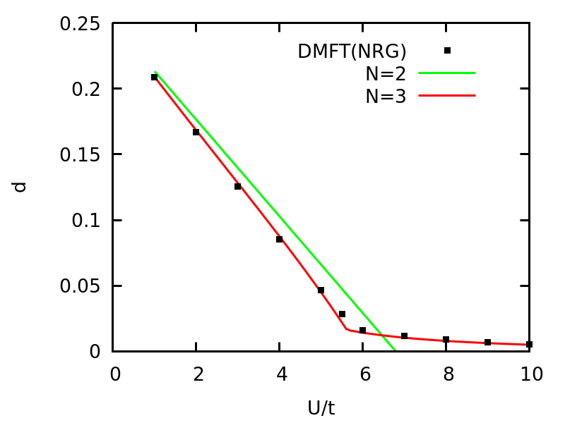
Now, we can easily solve this canonical model with N=2 and N=3 on a dense grid of U within seconds, and it is exciting to see the results. We use gnuplot to generate images. Using following commands, we can plot the double occupancy vs U and compare the VDAT results to DMFT with NRG solver.
VDATN3multi.jl/src/example/plot_one_band_half.gnuplot
Lines 11 to 15 in 2672897
The double occupancy vs U for one Hubbard model at half-filling on d=\infty Bethe lattice
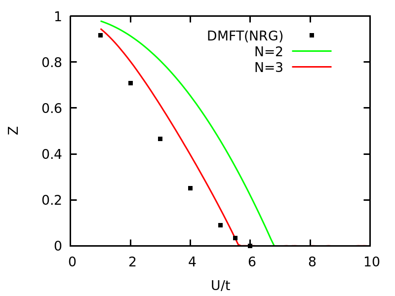
Using following commands, we can plot the quasi-particle weight Z vs U and compare the VDAT results to DMFT with NRG solver.
VDATN3multi.jl/src/example/plot_one_band_half.gnuplot
Lines 24 to 28 in 2672897
The quasi-particle weight Z vs U for one Hubbard model at half-filling on d=\infty Bethe lattice
One can simiply change n_target_ to solve the model at a given density (no magnetization). To simplify the process of generating data, we define the following functions:
VDATN3multi.jl/src/example/example_one_band_doped.jl
Lines 12 to 33 in 11f62b5
Then we could generate the solutions for a range of U and density as:
VDATN3multi.jl/src/example/example_one_band_doped.jl
Lines 36 to 47 in 11f62b5
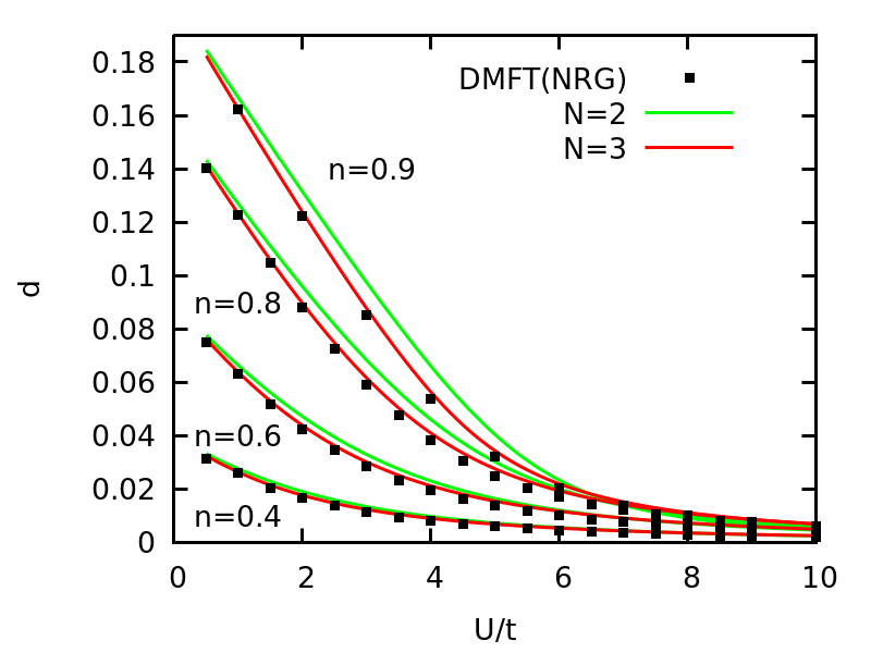
One can similarly perform the N=2 calculation. Finally, we check the double occupancy vs U using N=2 and N=3 and compare the result to DMFT(NRG).
It is also useful to solve the model at given chemical potential instead of given density.
VDATN3multi.jl/src/example/example_one_band_free.jl
Lines 9 to 21 in 7677f3f
Especially, one should pay attention to
which sets the model without any density constraint and pass a function named as cal_Eeff_U, which takes N_Ueff number of parameters to describe interacting projectors.The main purpose to introduce cal_Eeff is that for multi-orbital system, the number of variational parameters for interacting projectors grows exponentially with number of orbitals, and therefore, it is useful to let users to define customized ways to parametrize the interacting projectors. For example, cal_Eeff_U is defined as
Lines 168 to 185 in 7677f3f
The signature of cal_Eeff is (Γασ,μeffασ,Ueff_para), where Γασ is the atomic configuration, μeffασ is a rray of effective chemical potentials to control the densities, and Ueff_para is a array of effective interacting parameters to control the local correlations. cal_Eeff_U will become the Gutzwiller projector in the one-band case, and the probabilty of Γασ is proportional to exp(-cal_Eeff(Γασ,μeffασ,Ueff_para)). We also define
Line 122 in 7677f3f
to define the Jastrow projector when we have both U and J in multi-orbital case. It should be notes that N_Ueff is fixed for a given parametrization and must be passed to the model as illustrated above.
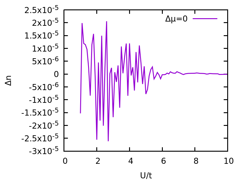
Now, we could solve the model with various chemical potentials at given U. First, it is useful to double-check results with the fixed density approach. We can set chemical potential as U/2, and compute density deviation from 0.5.
VDATN3multi.jl/src/example/example_one_band_free.jl
Lines 38 to 48 in 4af70df
The density deviation (i.e, n-0.5) vs U for one band Hubbard model using half-filling chemical potential.
One can understand that the deviation from the exact density is due to the error of numerical minization, and therefore, should relates to how the energy responses to the density deviation. For metal phase, energy is quadratic in density deviation while in insulating phase, it is linear in the absoluate value of density deviation. Therefore, we expect larger density deviation for the metal phase.
One can also check that two approaches produce the same double occupancy vs U plot:
Next, We start from half-filling parameters and increase chemical potential.
VDATN3multi.jl/src/example/example_one_band_free.jl
Lines 70 to 84 in 7677f3f
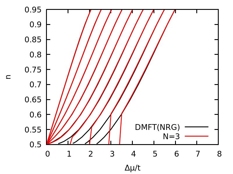
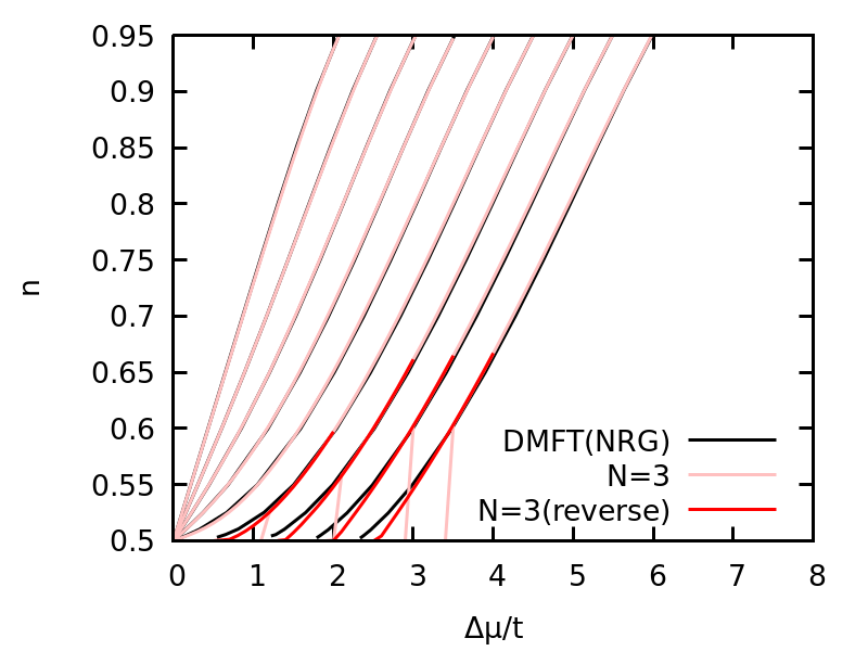
And we can plot the density as a function of chemical potential for U=1.0,2.0,...,9.0
The density as a function of chemical potential for U=1.0,2.0,...,9.0 for one-band Hubbard model. N=3(reverse) means that the calculation starts from a doped regime and decrease the chemical potential, while N=3 means the calculation starts from half-filling and increase the chemical potential.
Similar to the case with given chemical potential, we can solve the model at a given magnetic field.
VDATN3multi.jl/src/example/example_one_band_magnetic_field.jl
Lines 8 to 20 in c3e0a1b
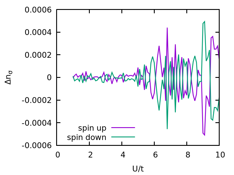
Here, we set chemical_potential_=[(1,U/2+B),(2,U/2-B)] so the total density is 1. We first check the results for B=0, which should yield n_up=n_dn=0.5. So we can plot the deviations of the dnesity for each spin orbital from the exact value.
We can also plot the deviation of the total density and magnetization from the exact value.
We can see the amplitude of deviations relates to the susceptibility of corresponding observables.
We can also check the double occupancy vs U/t with the fixed density approach.
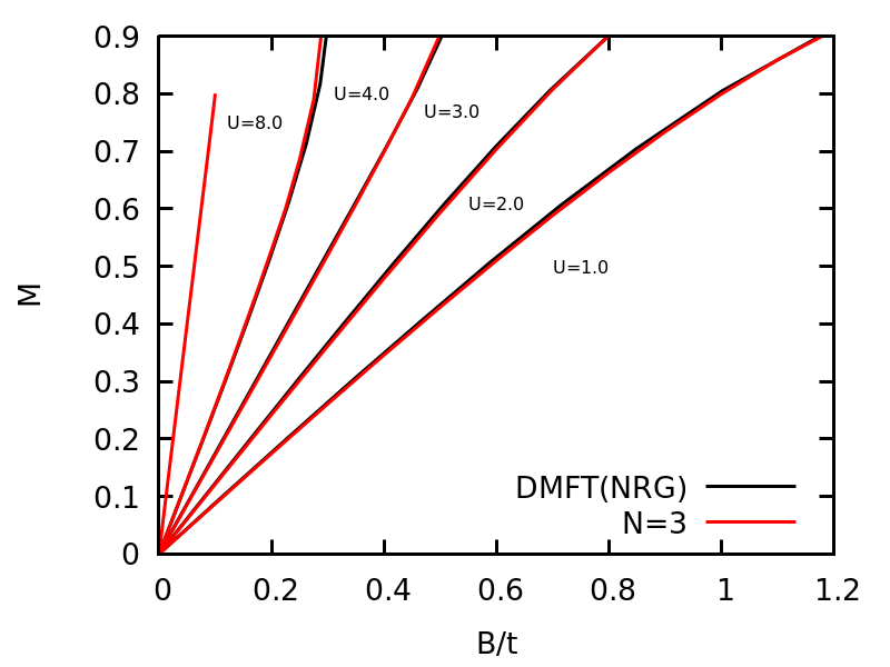
Finally, we can plot the magnetization vs B/t for various U. Here, we assume the magnetic field B coupldes to the system as -B*(n_up-n_dn) and the magnetization M is defined as M=n_up-n_dn
It is straightforward to generalize the above code to solve the multi-orbital problem. However, one should use more sophisticated parametrization of the local projector to ensure an efficient minimization. Based on experience, it turns out using Jastrow-like projector is much more stable than the fluctuation based projectors (the default way). In this part, we use a two-orbital Hubbard model to illustrate the ideas.
VDATN3multi.jl/src/example/example_two_band_half.jl
Lines 29 to 43 in da50ddd
Notice we should pass the following options to create_model: w_mode="fix",N_w_para_fixed=3,cal_w_fixed=cal_w_fixed_two_band_half The key function is cal_w_fixed_two_band_half, which is defined as
VDATN3multi.jl/src/example/example_two_band_half.jl
Lines 8 to 12 in da50ddd
In general, one should pass a function with signature (neffασ,w_para) -> w, where neffασ=(n1,n2,...,n_N_spin_orb) and the return value w should be constrained by neffασ. In addition, one should pass N_w_para_fixed, which is the size of w_para.
Now, we can solve a two-band Hubbard model with t1 and t2 as the hopping parameters for the first and second band.
To probe the metal insulator transition, we plot the quasi-particle weights for the two bands vs U.
t1/t2="0.2 0.3 0.4 0.5 0.6 0.7 0.8 0.9 1.0"

t1/t2="0.2 0.21 0.22 0.23 0.24 0.25 0.26 0.27 0.28 0.29 0.3"

t1/t2="0.1 0.11 0.12 0.13 0.14 0.15 0.16 0.17 0.18 0.19 0.2"

Interestingly, we find that for t1/t2 >=0.25, two bands simultaneously enter the Mott phase, where for t1/t2 <=0.25, two bands have two different transition values and the difference between two values increases when t1/t2 decreases.
We can also gain insights by inspecting the density-density correlation for different t1/t2.
In the previous section, we have discussed how the ratio of two bands, i.e, t1/t2, influences the transition value of MIT. Interestingly, we find that when t1/t2>0.25, two band have the same Uc, and when t1/t2<0.25, Uc for two bands becomes different, and system exhibits an orbital selective Mott transition. Moreover, when t1/t2->0, the second band behaves like an one-band model, while still have a non-trivial effect on the first band.
Now, we turn on J to see how J/U influences MIT. To parametrize the local projector, we introduce 4 independent interacting variational parameters.
VDATN3multi.jl/src/example/example_two_band_half_with_J.jl
Lines 20 to 23 in aa90445
Moreover, we pass J to generate the interactions (notice we ignore the spin-flip and pair-hopping terms)
VDATN3multi.jl/src/example/example_two_band_half_with_J.jl
Lines 45 to 52 in aa90445
Quasi-particle weight for first and second bands vs U/t2 for t1/t2=0.1, 0.2, 0.3, 0.4, 0.5, 0.6, 0.7, 0.8, 0.9, 1.0 and J/U=0.05
Interestingly, we found that the system has an orbital selective Mott transition (OSMT) when t1/t2<0.5, in constrast to the case of J/U=0 where t1/t2<0.25 is necessary for OMST.
Quasi-particle weight for first and second bands vs U/t2 for t1/t2=0.1, 0.2, 0.3, 0.4, 0.5, 0.6, 0.7, 0.8, 0.9, 1.0 and J/U=0.1
Quasi-particle weight for first and second bands vs U/t2 for t1/t2=0.1, 0.2, 0.3, 0.4, 0.5, 0.6, 0.7, 0.8, 0.9, 1.0 and J/U=0.25
We can see that when t1/t2<0.5, the transition for the first band is now become continuous. Moreover, for J/U=0.25 and t1/t2=0.1, the critical value of MIT for the first band is similar to the one-band critical value, i.e 5.6*0.1, but the second band still has non-trivial differences from one band behavior. To further explore these observations, we plot the density-density correlation functions vs U for various t1/t2 with J/U=0.25.
Density-density correlation functions vs U for t1/t2=0.9 with J/U=0.25.
Density-density correlation functions vs U for t1/t2=0.5 with J/U=0.25.
Density-density correlation functions vs U for t1/t2=0.1 with J/U=0.25.
