bbricks provides a collection of frequently used Bayesian parametric and nonparametric model structures, as well as a set of tools for common analytical tasks.
- Structures include linear Gaussian systems, Gaussian and Gaussian conjugate structure, Gaussian and Inverse-Wishart conjugate structure, Gaussian and Normal-Inverse-Wishart conjugate structure, Gaussian and Normal-Inverse-Gamma conjugate structure, Categorical and Dirichlet conjugate structure, Dirichlet Process on positive integers, Dirichlet Process in general, Hierarchical Dirichlet Process ...
- Tasks include updating posteriors, calculating marginal likelihood, calculating posterior predictive densities, sampling from posterior distribution, sampling from posterior predictive distribution, calculating MAP estimates ...
See Mindset for the idea behind bbricks and Examples to get started.
Note: This is a package designed for statisticians, and the ones who want to learn the basic Bayesian mindsets.
----Installation----
# install from CRAN:
install.packages("bbricks")
# or install development version from GitHub:
# install.packages("devtools")
devtools::install_github("chenhaotian/Bayesian-Bricks") - Hierarchical Bayesian Linear Regression
- Estimate Cancer Mortality Rates with Hierarchical Bayesian
- Mixture of Gaussian
- Hierarchical Mixture Models
- Hierarchical Mixture Models with Two Layers of Hierarchies
- Bayesian Linear Regression
- Hidden Markov Model (HMM)
- Infinite States Hidden Markov Model (HDP-HMM)
The idea of bbricks came from the fact that modeling in Bayesian statistics is nothing more than applying a set of tasks on a specific model structure.
Where the most frequently appeared tasks are:
- Update prior info into posterior when new samples are observed.
- Sample from the posterior distribution.
- Calculate marginal likelihood of the data set.
- Calculate posterior predictive densities from the posterior distribution.
- ...
And the model structures are always constituted by  basic Bayesian modeling structures:
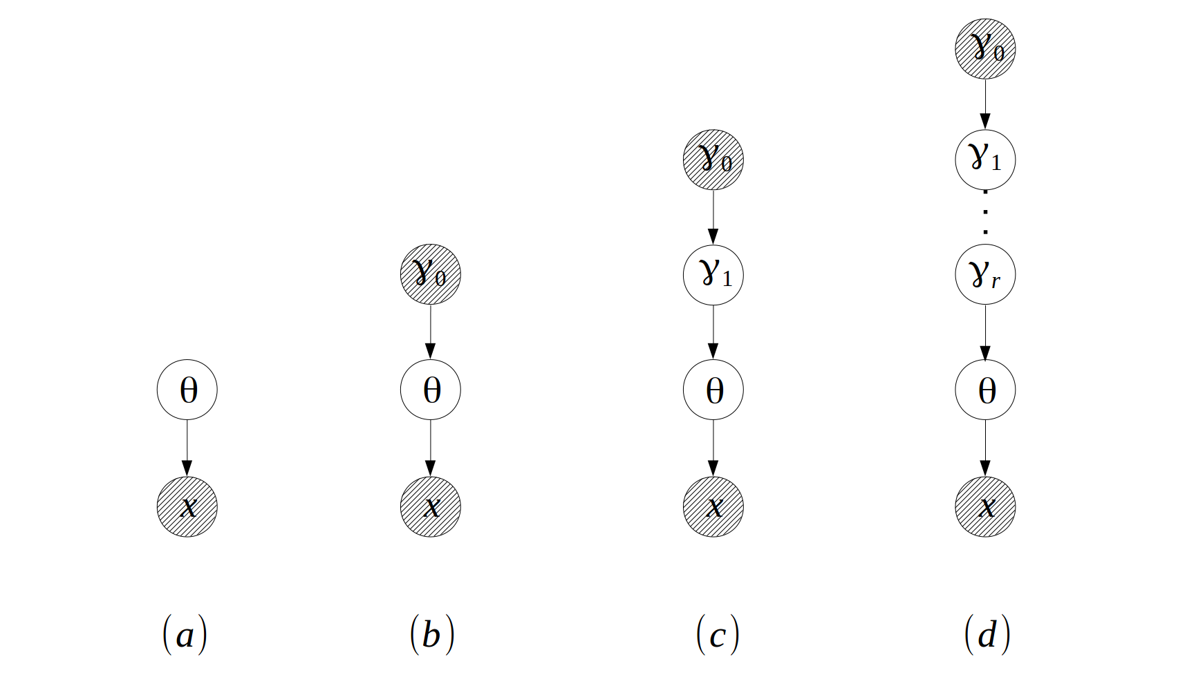 Where
Where
 is the most basic "parameter-observation" structure. Models like Gaussian, Gamma and Exponential are in this category.
 is the "prior-posterior" structure. Models like Gaussian-NIW(Gaussian observations with NIW prior), Categorical-Dirichlet(Categorical observations with Dirichlet prior) are in this category.
 is the "hierarchical-Bayesian" structure, and
  is the same hierarchical structure but with more hierarchies. Models like Hierarchical Dirichlet Process(HDP) and HDP with additional hidden layers are in this category.
bbricks tries to provide a type/class for each basic model structure and a function/method for each task.
See Examples for details.
This is an example from Hoff(2009). Where we want to examine the relationship between math score and another variable, socioeconomic status (SES) of students from  different schools. The Conditional Probability Distributions (CPDs) of the model are defined as:
Where  is the math score,
  is a length
  row vector
  corresponding to each math score observation in
  , NIW is Normal-Inverse-Wishart distribution, it's density function is defined as:
The graphical model structure for this model is:
To enable sampling from this model, we first look at the CPDs of the random variables and their Markov blankets:
- The Markov blanket for
 is
is  , the corresponding CPD of the blanket is a linear Gaussian system. bbricks provides an object of type
 "LinearGaussianGaussian"(see?LinearGaussianGaussianin R for details) to encode such a structure. - The Markov blanket for
 is
is  , the corresponding CPDs of the blanket forms an Gaussian-NIW conjugate structure. bbricks provides an object of type
 "GaussianNIW"(see?GaussianNIWin R for details) to encode such a structure. - The Markov blanket for
 is
is  , the corresponding CPDs of the blanket forms an Gaussian-InvWishart conjugate structure. bbricks provides an object of type
 "GaussianInvWishart"(see?GaussianInvWishartin R for details) to encode such a structure.
Note that "LinearGaussianGaussian", "GaussianNIW" and "GaussianInvWishart" are all basic prior-posterior structure as shown in Mindset graph  . In bbricks, all objects representing structures same as graph
  are also of type
 "BasicBayesian". For example a "LinearGaussianGaussian" object is also an "BasicBayesian" object.
To estimate the posterior parameters  , the Gibbs sampling procedure goes as:
- Sample
 from a
 LinearGaussianGaussianobject which encodes the distribution of .
. - Sample
 from a
 GaussianNIWobject which encodes the distribution of
- Sample
 from a
 GaussianInvWishartobject which encodes the distribution of
R code:
## Gibbs sampling for hierarchical linear regression

library(bbricks)
## load some hierarchical linear regression data
## hlrData is a list of 3 numeric vectors
## see ?hlrData for details
data(hlrData)
x <- hlrData$mathScore                    #math score as the dependent variable
X <- cbind(1,hlrData$socioeconomicStatus) #socioeconomic status as the independt variable
js <- hlrData$schoolID                    #school ID as the group IDs.
J <- max(js)
## Initialization----------------------------------------------
## initialize the Markov blanket of mu and Sigma
## the prior parameters are: m=0, k=0.0001, v=3, S=diag(1)
objmS <- GaussianNIW(gamma = list(m =c(mean(hlrData$mathScore),0),k=0.0001,v=3,S=diag(2)))
## initialize the Markov blanket of sigma^2
## the prior parameters are: vs=2, Ss=diag(1)
objs <- GaussianInvWishart(gamma = list(mu=0,v=2,S=diag(1)))
## initialize mu and Sigma by sampling from the prior
muSigma <- rPosterior(objmS)
## initialize sigma^2 by sampling from the prior
sigma2 <- rPosterior(objs)
betaJ <- matrix(0,J,2)                  #place-holder the beta_j, j=1:J
epsilon <- x                            #place-holder for the random noises
## Main Gibbs loop---------------------------------------------
maxit <- 100                           #number of sampling iterations
burnin <- 50                           #number of burn-in samples
meanBeta <- betaJ                      #place-hoder for the sample means of beta
it <- 1
pb <- txtProgressBar(min = 0,max = maxit,style = 3)
while(it<=maxit){
    ## Step1: sample beta_j, j in 1:100
    for(j in 1L:J){
        objb <- LinearGaussianGaussian(gamma=list(Sigma=sigma2,m=muSigma$mu,S=muSigma$Sigma))
        idx <- js == j
        ss <- sufficientStatistics(obj = objb,x=x[idx],A=X[idx,,drop=FALSE])
        posterior(obj = objb,ss = ss)
        betaJ[j,] <- rPosterior(objb)
    }
    ## calculate the sample mean
    if(it>burnin) meanBeta <- meanBeta+betaJ/(maxit-burnin)
    ## Step2: sample mu and Sigma
    ssmS <- sufficientStatistics(obj = objmS,x=betaJ)
    posterior(obj = objmS,ss = ssmS)
    muSigma <- rPosterior(obj = objmS)
    ## Step3: sample sigma^2
    for(j in 1L:J){
        idx <- js == j
        epsilon[idx] <- x[idx]-X[idx,,drop=FALSE]%*%betaJ[j,]
    }
    sss <- sufficientStatistics(obj = objs,x=epsilon)
    posterior(obj = objs,ss = sss)
    sigma2 <- rPosterior(objs)
    ## increase iteration counter
    it <- it+1
    setTxtProgressBar(pb,it)
    ## if continue sampling, then discard the information in objmS and objs
    ## to make room for the new information in the next iteration.
    if(it < maxit){
        posteriorDiscard(obj = objmS,ss = ssmS)
        posteriorDiscard(obj = objs,ss = sss)
    }
}
## plot the result
## gray lines are the betas of each school
## black line is the beta for all the data as a whole
plot(x=0, xlim = range(0.2,0.8),ylim = c(20,35),xlab = "socioeconomic status",ylab = "math score")
for(j in 1L:J)
    abline(a=betaJ[j,2],b=betaJ[j,1],col="gray")
allSchools <- lm(x~X-1)$coefficients
abline(a=allSchools[2],b=allSchools[1],lwd=3)
This is an example from Johson and Albert(2006), where we want to estimate the cancer mortality rates of multiple cities with hierarchical Bayesian method.
The model's graph structure is:
Where  is a categorical random sample that takes one of two values: "death" or "no death". There are
  cities in total,
  are the mortality rates of the cities.
The CPDs are:
To enable sampling from this model, we first look at the CPDs of the random variables and their Markov blankets:
- The Markov blanket for
 is
is  , the corresponding CPD of the blanket is a Categorical-Dirichlet conjugate structure. bbricks provides an object of type
 "CatDirichlet"(see?CatDirichletin R for details) to encode such a structure. - The Markov blanket for
 is
is  , the corresponding CPDs of the blanket is not very common thus not provided in bbricks, instead we can use Metropolis-Hastings algorithm to sample from it.
Note that "CatDirichlet" is a basic prior-posterior structure as shown in Mindset graph  . In bbricks, all objects representing structures same as graph
  are also of type
 "BasicBayesian". For example a "CatDirichlet" object is also an "BasicBayesian" object.
To estimate  , we use the following Gibbs sampling procedure:
- sample
 from a
 CatDirichletobject which encodes the distribution of .
. - sample
 from the distribution of
  with and independent Metropolis-Hastings algorithm. see
 ?MetropolisHastingsfor details.
R code:
## Estimate cancer mortality rates using Gibbs sampling

library(bbricks)

## see ?cancerData for details
data(cancerData)
## Step1: Initialization----------------------------------------------
K <- length(cancerData)                          #then number of cities
eta <- 1                                         #assume eta is known, eta=1
## initialize alpha, PI, and sufficient statistics
a <- rexp(2,rate = eta)                 #initialize alpha
PI <- matrix(0,K,2L)                    #initialize pi
cityPrior <- CatDirichlet(gamma = list(alpha=a,uniqueLabels=c("death","no death")))
citySS <- lapply(cancerData,function(x){sufficientStatistics(obj = cityPrior,x=x)}) #sufficient statistics of each city
## initialize functions used in Metropolis-Hastings, see ?MetropolisHastings for details
## density of the target distribution
dp <- function(a){
    if(any(a<0)) -Inf
    else sum(dDir(x=PI,alpha = a,LOG = TRUE))+sum(dexp(x=a,rate = eta,log = TRUE))
}
## density of the proposal distribution
dq <- function(anew,a){1}                #use a independent proposal
## random sample generator of the proposal distribution
rq <- function(x){
    c(runif(1,x[1]-1,x[1]+1),
      runif(1,x[2]-1,x[2]+1))
}
## Step2: main Gibbs sampling loop between alpha and pi --------------
maxit <- 1000
burnin <- 500                            #number of burn-in samples
meanPI <- numeric(K)                     #place-hoder for the sample mean
it <- 1
while(it<=maxit){
    ## Step1: sample pi from p(pi|a,x)-------------
    for(k in 1L:K){
        posterior(obj = cityPrior,ss=citySS[[k]])
        PI[k,] <- rDir(n=1,alpha = cityPrior$gamma$alpha)
        posteriorDiscard(obj = cityPrior,ss=citySS[[k]])
    }
    ## calculate the sample mean
    if(it>burnin) meanPI <- meanPI+PI[,1]/(maxit-burnin)
    ## Step2: sample a from p(a|pi,g)--------------
    ## use Metropolis-Hastings
    a <- MetropolisHastings(nsamples = 1,xini = a,dp=dp,dq=dq,rq=rq)
    ## increase iteration counter
    it <- it+1
}
## Step3: plot the result---------------------------------------------
## black bars are the sample mean from the hierarchical Bayesian model
## blue bars are the MLE of the mortality rates.
plot(1:K,meanPI,type = "h",xlab = "city",ylab = "mortality rate",lwd=3)
lines(1:K+0.2,sapply(cancerData,function(l){sum(l=="death")/length(l)}),type = "h",col = "blue",lwd = 3)
legend(1, 0.005, legend=c("Sample Mean", "MLE"),col=c("black", "blue"), lty=c(1,1), cex=1,lwd = 3) A mixture of Gaussian has the following graph structure:
Where there are  Gaussian components/groups.
  is an Gaussian observation,
  is the hidden group label,
  is the component weights (or the group label distribution).
  are the observation distribution parameters.
  and
and  are prior parameters.
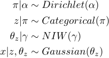
The CPDs are:
Where  is the Normal-Inverse-Wishart distribution with parameter
  .
.  is a numeric vector representing the "location parameter",
  is a symmetric positive definitive matrix representing the "scale parameter",
  and
and  are degree of freedoms. For a NIW sample
  , it's density function is defined as:
A mixture model can be see as a combination of two "prior-posterior" structures(As shown in Mindset graph  ): One Categorical-Dirichlet structure
  for the hidden cluster labels. and one Gaussian-NIW structure
  for the observation distribution.
In bbricks these two structures are initialized with a "CatDirichlet" object and a "GaussianNIW" object. To estimate  and
and  , we use the following EM procedure:
- E-step: calculate
 and the expected sufficient statistics
 and
and  .
. - M-step: Based on the expected sufficient statistics to get an MAP estimate of
 and
and 
R code:
## Get the MAP estimate of pi and theta using EM algorithm.

library(bbricks)

## load some mixture of Gaussian samples.
## mmData is a numeric matrix with 2 columns, each row is a sample
## see ?mmData for details
data(mmData)
K <- 4L                                 #number of clusters(mixtures components)
z <- matrix(runif(nrow(mmData)*K),nrow(mmData),K) #the expected cluster label of each observation
allK <- 1L:K    #temp variable, all component labels
allZ <- rep(allK,each=nrow(mmData))     #temp variable, all possible cluster labels for all observations
## z, pi and alpha are distributed as a Categorical-Dirichlet sturcture:
mc <- CatDirichlet(gamma = list(alpha=0.5,uniqueLabels=allK)) # create a CatDirichlet object to track the posterior info, see ?CatDirichlet for details
## each component distribution is a Gaussian-NIW structure:
ec <- replicate(K,GaussianNIW(gamma = list(m=c(0,0),k=0.00001,v=2,S=diag(2)))) # create a GaussianNIW object to track the posterior info of each mixture component, see ?GaussianNIW for details
mcMAP <- MAP(mc)                        #initialize the MAP estimate of pi
ecMAP <- replicate(K,list(muMAP=runif(2),sigmaMAP=diag(2)),simplify = FALSE) #initialize the MAP estimate of theta
## The main EM loop
maxit <- 100                            #number of EM loops
it <- 1
while(it<=maxit){
    ## E-step---------------------------------------------------------
    ## calculate the expected cluster labels: p(z|pi,theta)
    for(k in allK) z[,k] <- dGaussian(x=mmData,mu = ecMAP[[k]]$muMAP,Sigma=ecMAP[[k]]$sigmaMAP)+log(mcMAP[k])
    z <- exp(z-logsumexp(z))            #use logsumexp() to avoid numerical underflow
    ## calculate the expected sufficient statistics
    ssComponents <- lapply(allK,function(k){
        sufficientStatistics_Weighted(obj = ec[[k]],x=mmData,w=z[,k])
    })                                  #the expected sufficient statistics of each Gaussian component
    ssPi <- sufficientStatistics_Weighted(obj = mc,x=allZ,w=as.vector(z)) #the expected sufficient statistics of the cluster label distribution
    ## M-step---------------------------------------------------------
    ## use the sufficient statistics to update the prior distributions:
    for(k in allK) posterior(obj = ec[[k]],ss=ssComponents[[k]]) #update component distributions
    posterior(obj = mc,ss = ssPi)                                #update cluster label distribution
    ## calculate the MAP estimates from posterior:
    mcMAP <- MAP(mc)
    ecMAP <- lapply(ec,MAP)
    ## Reset the priors for next EM loop-----------------------------------------
    ## to prepare for the next EM iteration, discard the sufficient statistics info from the posteriors:
    for(k in allK) posteriorDiscard(obj = ec[[k]],ss=ssComponents[[k]])
    posteriorDiscard(obj = mc,ss = ssPi)
    ## increase the iteration counter
    it <- it+1
}

plot(mmData,col=apply(z,1,which.max)) #plot the best estimates
mcMAP                                 #the MAP estimate of pi
ecMAP #the MAP estimate of theta_z The graph structure of Dirichlet Process Mixture Model(DP-MM) is exactly the same as a standard mixture model, except that the number of mixture components is not predetermined:
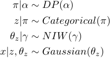
The CPDs of a DP-MM is similar to the ones shown in Mixture of Gaussian, the only difference is the distribution of  is a Dirichlet process rather than a Dirichlet distribution, for example if the observations are Gaussian distributed, the CPDs will be:
Where  is a Dirichlet process on positive integers with "concentration parameter"
  , the "base measure", which is an uniform distribution on positive integers, is omitted from the formula.
  is the Normal-Inverse-Wishart distribution with parameter
  .
.  is a numeric vector representing the "location parameter",
  is a symmetric positive definitive matrix representing the "scale parameter",
  and
and  are degree of freedoms.
A DP-MM can be see as a combination of two "prior-posterior" structures(As shown in Mindset graph  ): One Categorical-DirichletProcess structure for the hidden cluster label distribution
  , which we call it a "DP on positive integers". And one structure for the observation distribution
  .
.
In bbricks, "DP on positive integers" is represented by an object of type "CatDP".
To further simplify the calculations, bbricks also provides an "DP" type to represent all Dirichlet process structures. An object of type "DP" is in essence a combination of a "CatDP" object, which encodes the  structure, i.e. a Dirichlet process on positive integers, and an arbitrary
 "BasicBayesian" object, which encodes the  structure. (in bbricks, all models with same structure as Mindset graph
  are
are "BasicBayesian" s, such as "GaussianNIW", "GaussianNIG", "CatDirichlet" and even "CatDP") .
To estimate  , we use the following collapse Gibbs sampling procedure:
R code:
## Learn DP-MM posteriors using Gibbs sampling

library(bbricks)

## load some mixture of Gaussian samples.
## mmData is a numeric matrix with 2 columns, each row is a sample
## see ?mmData for details
data(mmData)
maxit <- 100                            #number of total samples
burnin <- 50                            #number of burnin samples
## Step1: Initialization -----------------------------------------
obj <- DP(gamma = list(alpha=10,H0aF="GaussianNIW",parH0=list(m=c(0,0),k=0.001,v=2,S=diag(2)))) #create a DP object to track all the changes, the DP object in this case is a combination of a CatDP object and a GaussianNIW object
z <- matrix(1L,nrow(mmData),maxit-burnin)    #place-holder for the sampled z
ss <- sufficientStatistics(obj,x=mmData,foreach = TRUE) #sufficient statistics of each observed sample
N <- nrow(mmData)
for(i in 1L:N){ # initialize labels before Gibbs sampling
    z[i,1] <- rPosteriorPredictive(obj = obj,n=1,x=mmData[i,,drop=FALSE])
    posterior(obj = obj,ss = ss[[i]], z = z[i,1])
}
## Step2: Main Gibbs sampling loop--------------------------------
it <- 1                                 #iteration tracker
pb <- txtProgressBar(min = 0,max = maxit,style = 3)
while(it<=maxit){
    if(it>burnin) colIdx <- it-burnin
    else colIdx <- 1
    for(i in 1L:N){
        ## remove the sample information from the posterior
        posteriorDiscard(obj = obj,ss = ss[[i]],z=z[i,colIdx])
        ## get a new sample
        z[i,colIdx] <- rPosteriorPredictive(obj = obj,n=1,x=mmData[i,,drop=FALSE])
        ## add the new sample information to the posterior
        posterior(obj = obj,ss = ss[[i]],z=z[i,colIdx])
    }
    if(it>burnin & colIdx<ncol(z)) z[,colIdx+1] <- z[,colIdx] #copy result of previous iteration
    it <- it+1
    setTxtProgressBar(pb,it)
    if(it>=maxit){cat("\n");break}
    plot(x=mmData[,1],y=mmData[,2],col=z[,colIdx]) #to see how the labels change in each iteration
}
## Step3: Estimate group labels of each observation---------------
## pick the most frequent z as the best estimate
zBest <- apply(z,1,function(l){
    tmp <- table(l)
    names(tmp)[which.max(tmp)]
})
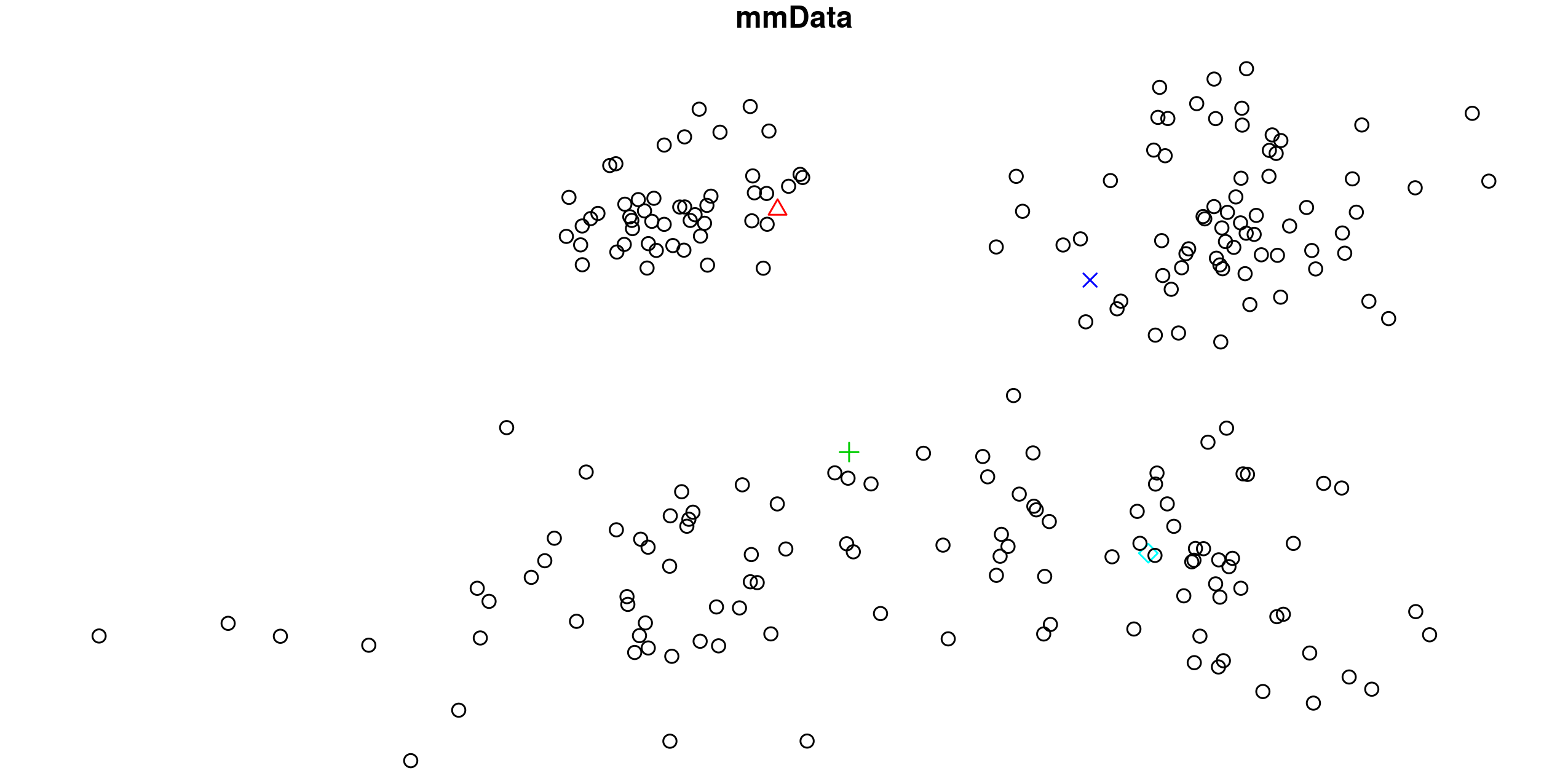
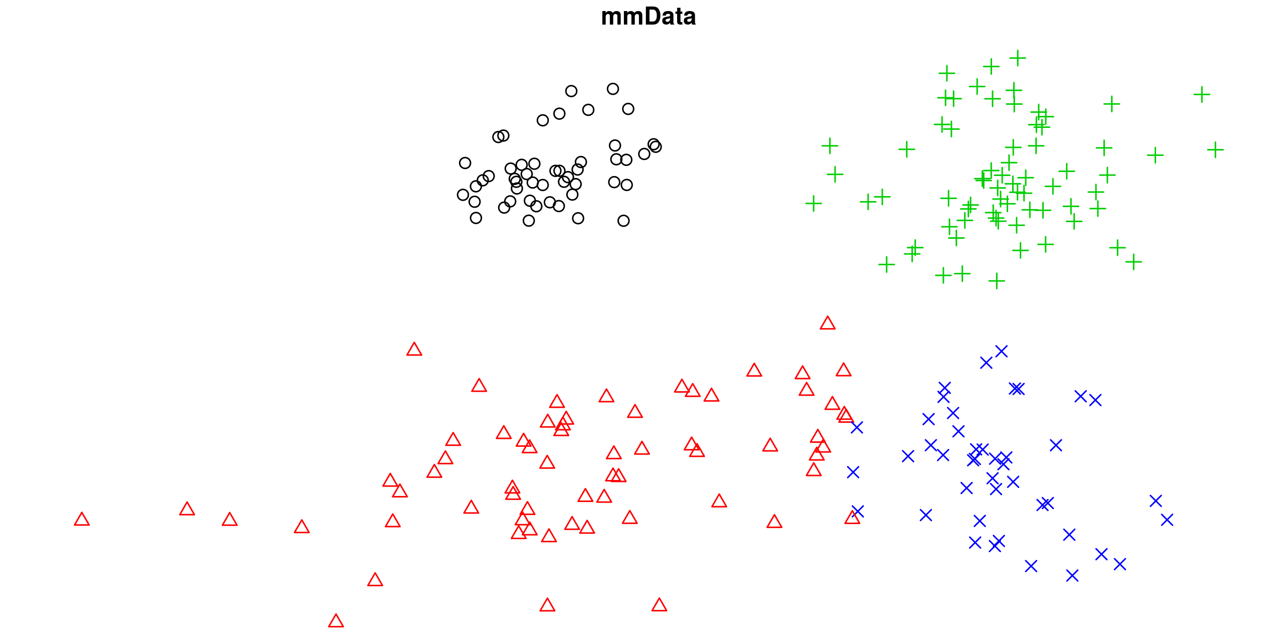
plot(x=mmData[,1],y=mmData[,2],col=zBest) In the dataset mmData of the previous example, what if we know the 50, 100, 150 and 200th samples belong to 4 different clusters(they are shown as different color and shapes in the graph below), how should we incorporate this information in the model?
With DP-MM, one only need to 1. update the DP prior (as defined in previous R example) with the information of the 4 observed samples, and 2. use the updated prior as the prior of the Gibbs sampling procedure. These 2 steps can be achieved by adding following code after obj <- DP(...) in the previous R example:
## 1. add the information of the 4 observed samples to the DP object
ssObserved <- sufficientStatistics(obj=obj,x=mmData[c(50,100,150,200),,drop=FALSE],foreach = TRUE)
for(i in 1L:4L) posterior(obj = obj,ss = ssObserved[[i]], z = i) # the choice of cluster label 'z' for the 4 observed samples are arbitrary, as long as they are different from each other. In this example I simply use z=1L:4L.
## 2. remove the 4 samples from the upcoming Gibbs sampling procedure
mmData <- mmData[-c(50,100,150,200),]
Run the code, and the result will be:
In a hierarchical mixture model, the observation  are generated by some unknown mixture components and are split into
  groups, all
  groups share the same set of mixture components but with different mixture weights.
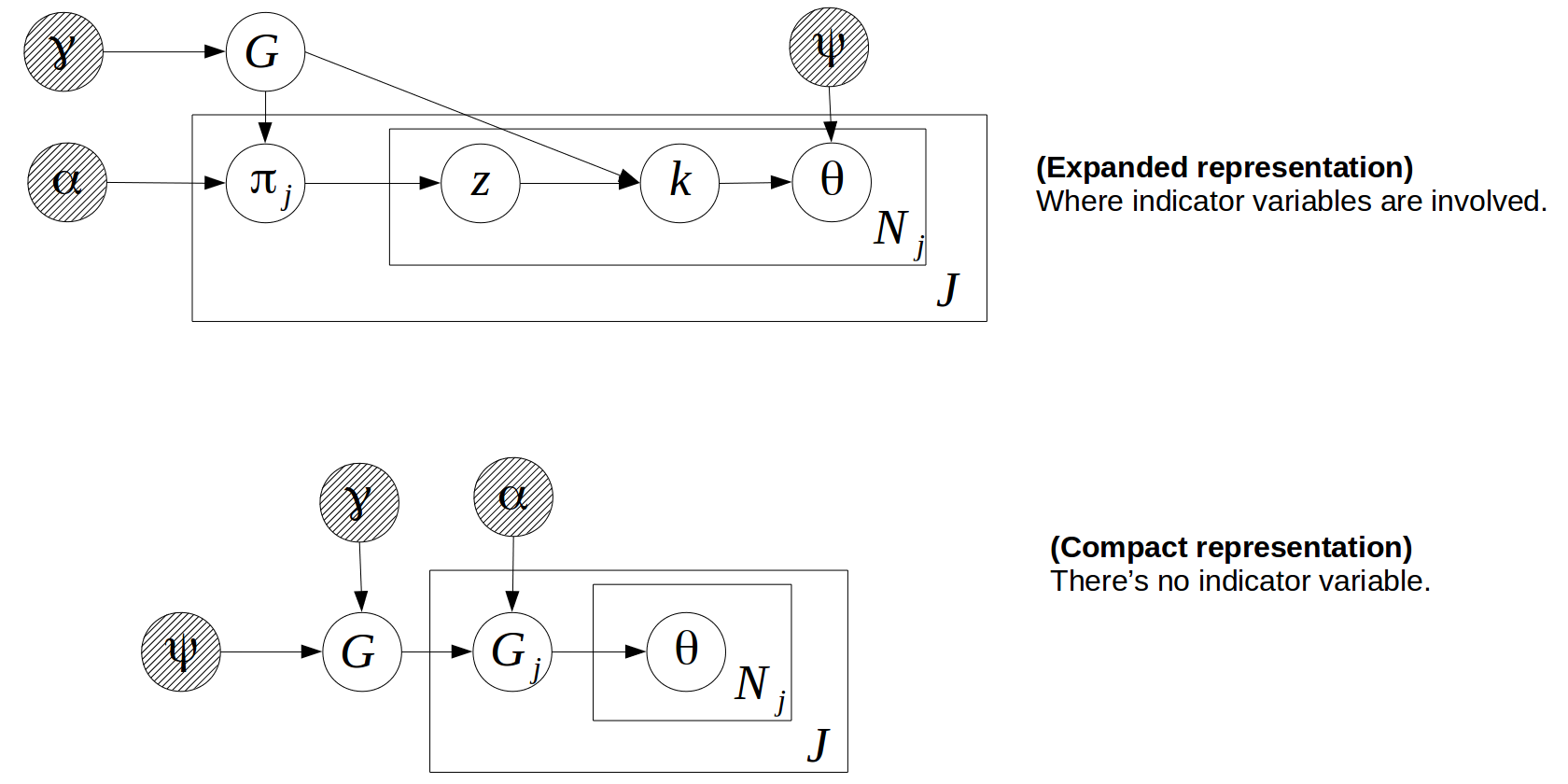
Hierarchical Dirichlet Process(HDP) is a natural representation of a hierarchical mixture model, It has following graph structure:
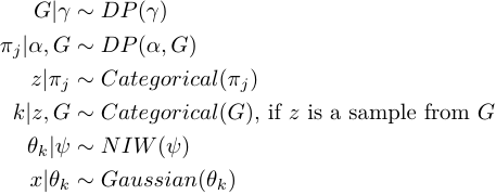
If the component distribution is Gaussian, the CPDs will be:
Where  is a Dirichlet process on positive integers with "concentration parameter"
  , the "base measure", which is an uniform distribution on positive integers, is omitted from the formula.
  is a Dirichlet process with concentration parameter
  and base measure
  .
.  is the Normal-Inverse-Wishart distribution with parameter
  .
.  is a numeric vector representing the "location parameter",
  is a symmetric positive definitive matrix representing the "scale parameter",
  and
and  are degree of freedoms.The distribution of
  is a "HDP on positive integers".
HDP are usually represented in a much simpler and compact way(though not easier to use in practice, especially when generating random samples from HDP) in most literature:
From the compact representation we can see that HDP is following the "Hierarchical Bayesian" structure shown in Mindset graph  .
.
In bbricks, "HDP on positive integers" is represented by an object of type "CatHDP". To further simplify the mixture model calculations, bbricks alos provides an "HDP" type to represent more general hierarchical Dirichlet process models. An object of type "HDP" is in essence a combination of a "CatHDP" object, which encodes the distribution of  , i.e. a HDP on positive integers; and an arbitrary
 "BasicBayesian" object, which encodes the  structure. (in bbricks, all models with same structure as Mindset graph
  are
are "BasicBayesian" s, such as "GaussianNIW", "GaussianNIG" ,"CatDirichlet" and even "CatDP")
To estimate  , we use the following Gibbs sampling procedure:
R code:
## Learn HDP-MM posteriors using Gibbs sampling

library(bbricks)

## load some mixture of Gaussian samples.
## mmhData is a list of two elements. mmhData$x is a matrix of Gaussian observations, each row is an observation; mmhData$groupLabel is the group label of each observation.
## see ?mmhData for details
data(mmhData)
x <- mmhData$x
js <- mmhData$groupLabel
## Step1: Initialization------------------------------------------
maxit <- 50                             #iterative for maxit times
burnin <- 30                            #number of burn in samples
## create a HDP object to track all the changes, the HDP object in this case is a combination of a CatHDP object and a GaussianNIW object:
obj <- HDP(gamma = list(gamma=1,j=max(js),alpha=1,
                        H0aF="GaussianNIW",
                        parH0=list(m=c(0,0),k=0.001,v=2,S=diag(2)*0.01)))
ss <- sufficientStatistics(obj$H,x=x,foreach = TRUE) #sufficient statistics
set.seed(1)
z <- rep(1L,nrow(x))
k <- matrix(1L,nrow(x),maxit-burnin)    #place-holder for the sampled k
N <- length(ss)
for(i in 1L:N){# initialize k and z
    tmp <- rPosteriorPredictive(obj = obj,n=1,x=x[i,,drop=FALSE],j=js[i])
    z[i] <- tmp["z"]
    k[i,1] <- tmp["k"]
    posterior.HDP(obj = obj,ss = ss[[i]],ss1 = k[i],ss2 = z[i],j = js[i])
}
## Step2: main Gibbs loop---------------------------------------------
it <- 1                                 #iteration tracker
pb <- txtProgressBar(min = 0,max = maxit,style = 3)
while(it<=maxit){
    if(it>burnin) colIdx <- it-burnin
    else colIdx <- 1
    for(i in 1L:N){
        ## remove the sample from the posterior info
        posteriorDiscard(obj = obj,ss = ss[[i]],ss1=k[i,colIdx],ss2=z[i],j=js[i])
        ## resample a new partition
        tmp <- rPosteriorPredictive(obj = obj,n=1,x=x[i,,drop=FALSE],j=js[i])
        z[i] <- tmp["z"]
        k[i,colIdx] <- tmp["k"]
        ## add the information of the new sample
        posterior(obj = obj,ss = ss[[i]], ss1=k[i,colIdx],ss2 = z[i],j=js[i])
    }
    if(it>burnin & colIdx<ncol(k)) k[,colIdx+1] <- k[,colIdx] #copy result of previous iteration
    it <- it+1
    plot(x=x[,1],y=x[,2],col=k[,colIdx])         #to visualize the group label dynamics
    setTxtProgressBar(pb,it)
}
## Step3: Estimate group labels of each observation---------------
## pick the most frequent k as the best estimate
kBest <- apply(k,1,function(l){
    tmp <- table(l)
    names(tmp)[which.max(tmp)]
})
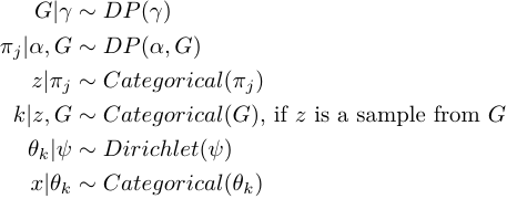
plot(x=x[,1],y=x[,2],col=kBest) A topic model is a hierarchical mixture model(See Hierarchical Mixture Models) with categorical component distribution:
The Gibbs sampling procedure on this model is exactly the same as the one in Hierarchical Mixture Models
R code:
## Learn HDP-LDA posteriors of the farm-ads corpus

## load a subset of farm ads data from https://archive.ics.uci.edu/ml/datasets/Farm+Ads
## see ?farmadsData for details
data(farmadsData)
word <- farmadsData$word
document <- farmadsData$document
## Step1: Initialization------------------------------------------
set.seed(1)
maxit <- 30                            #iterative for maxit times
z <- rep(1L,length(word))
k <- rep(1L,length(word))
## initialize
uniqueWords <- unique(word)
obj <- HDP(gamma = list(gamma=1,j=max(document),alpha=1,H0aF="CatDirichlet",parH0=list(alpha=rep(0.5,length(uniqueWords)),uniqueLabels=uniqueWords))) #create a HDP object to track all the changes, the HDP object in this case is a combination of a CatHDP object and a CatDrirchlet object
N <- length(word)
## initialize k and z
for(i in 1L:N){
    tmp <- rPosteriorPredictive(obj = obj,n=1,x=word[i],j=document[i])
    z[i] <- tmp["z"]
    k[i] <- tmp["k"]
    posterior(obj = obj,ss = word[i], ss2 = z[i],j=document[i],ss1=k[i])
}
## Step2: main Gibbs loop---------------------------------------------
it <- 1                                 #iteration tracker
pb <- txtProgressBar(min = 0,max = maxit,style = 3)
while(it<=maxit){
    for(i in 1L:N){
        posteriorDiscard.HDP(obj = obj,ss = word[i],ss1=k[i],ss2=z[i],j=document[i]) #remove the sample information from the posterior
        tmp <- rPosteriorPredictive(obj = obj,n=1,x=word[i],j=document[i])   #get a new sample
        z[i] <- tmp["z"]
        k[i] <- tmp["k"]
        posterior(obj = obj,ss = word[i],ss1=k[i], ss2 = z[i],j=document[i]) #add the new sample information to the posterior
    }
    it <- it+1
    setTxtProgressBar(pb,it)
}
## Step3: plot the result --------------------------------------------
## see which topics are most frequently appeared:
order(sapply(obj$X,function(l){sum(l$gamma$alpha)}),decreasing = TRUE)
## seems topic 2 and 1 appear the most, let's plot them:
## install.packages("wordcloud") # for word-cloud
## install.packages("RColorBrewer") # color palettes
## print topic 1
wordcloud:: wordcloud(words = obj$X[[1]]$gamma$uniqueLabels,
                      freq = obj$X[[1]]$gamma$alpha,
                      min.freq = 1,
                      max.words=100,
                      random.order=FALSE, rot.per=0.35,
                      colors=RColorBrewer::brewer.pal(5, "Set1"))
## print topic 2
wordcloud:: wordcloud(words = obj$X[[2]]$gamma$uniqueLabels,
                      freq = obj$X[[2]]$gamma$alpha,
                      min.freq = 1,
                      max.words=100,
                      random.order=FALSE, rot.per=0.35,
colors=RColorBrewer::brewer.pal(5, "Set1")) By extending the Hierarchical Mixture Models with an additional layer of Dirichlet process on top, the model is then able to capture longer-term and cross-group dependencies.
In this hierarchical mixture model, the observation  are generated by some unknown mixture components and are split into
  groups, each group has
  sub-groups. All
  groups share the same set of mixture components but with different mixture weights, all
  sub-groups within each group
  also share the same set of mixture components but different mixture weights. The graphical model structure is:
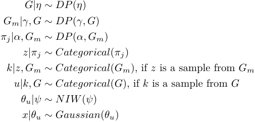
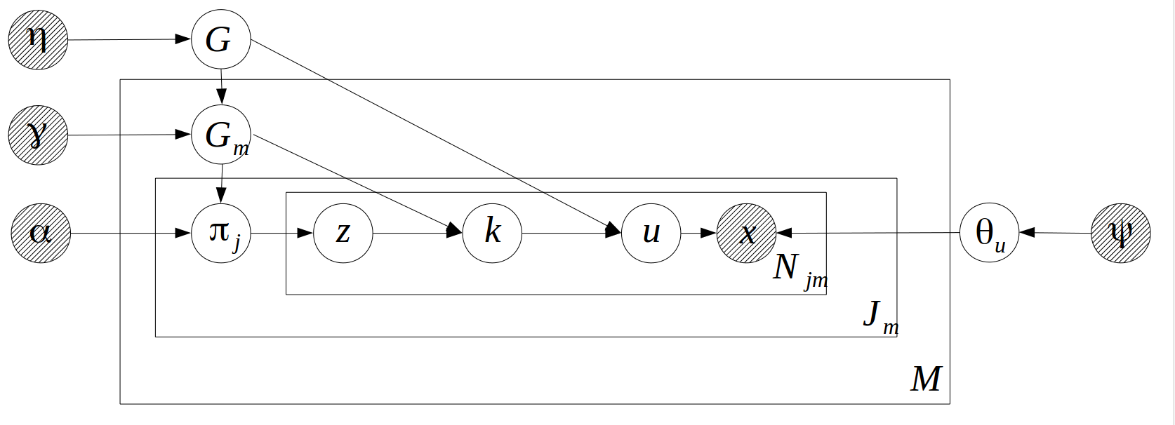 If the component distribution is Gaussian, the CPDs will be:
Where  is a Dirichlet process on positive integers with "concentration parameter"
  , the "base measure", which is an uniform distribution on positive integers, is omitted from the formula.
  is a Dirichlet process with concentration parameter
  and base measure
  .
.  is a Dirichlet process with concentration parameter
  and base measure
  .
.  is the Normal-Inverse-Wishart distribution with parameter
  .
.  is a numeric vector representing the "location parameter",
  is a symmetric positive definitive matrix representing the "scale parameter",
  and
and  are degree of freedoms.
The distribution of  is a "HDP on positive integers with two layers of hierarchies". Like the
 "CatHDP" object mentioned in Hierarchical Mixture Models, bbricks use a "CatHDP2" object to represent a "HDP on positive integers with two layers of hierarchies".
To simplify the mixture model calculations, bbricks also provides an "HDP2" type to represent all hierarchical Dirichlet process with two layers of hierarchies. An object of type "HDP2" is in essence a combination of a "CatHDP2" object, which encodes the distribution of  , i.e. a HDP on positive integers with two layers of hierarchies; and an arbitrary
 "BasicBayesian" object, which encodes the  structure. (in bbricks, all models with same structure as Mindset graph
  are
are "BasicBayesian" s, such as "GaussianNIW", "GaussianNIG", "CatDirichlet" and even "CatDP")
To estimate  , we use the following Gibbs sampling procedure:
R code:
## Learn HDP2-MM posteriors using Gibbs sampling

library(bbricks)

## load some mixture of Gaussian samples.
## mmhData is a list of 3 elements. mmhhData$x is a matrix of Gaussian observations, each row is an observation; mmhhData$groupLabel is the group label of each observation. mmhhData$subGroupLabel is the subgroup label of each observation.
## there are 2 groups, group1 has 10 subgroups, group has 20 subgroups.
## see ?mmhhData for details
data(mmhhData)
x <- mmhhData$x
groupLabel <- mmhhData$groupLabel
subGroupLabel <- mmhhData$subGroupLabel
## Step1: Initialization------------------------------------------
maxit <- 50                            #iterative for maxit times
burnin <- 20                           #number of burn in samples
## create a HDP2 object to track all the changes, the HDP2 object in this case is a combination of a CatHDP2 object and a GaussianNIW object
obj <- HDP2(gamma = list(eta=1,gamma=1,alpha=1,m=2L,j=c(10L,20L),H0aF="GaussianNIW",parH0=list(m=c(0,0),k=0.001,v=1.1,S=diag(2)*0.001)))
ss <- sufficientStatistics(obj$H,x=x,foreach = TRUE) #sufficient statistics
z <- rep(1L,nrow(x))
k <- rep(1L,nrow(x))
u <- matrix(1L,nrow(x),maxit-burnin)
N <- length(ss)
## initialization k, z and u
for(i in 1L:N){
    tmp <- rPosteriorPredictive(obj = obj,n=1,x=x[i,,drop=FALSE],m=groupLabel[i],j=subGroupLabel[i])
    z[i] <- tmp["z"]
    k[i] <- tmp["k"]
    u[i,1] <- tmp["u"]
    posterior.HDP2(obj = obj,ss = ss[[i]],ss1 = u[i,1],ss2 = k[i],ss3 = z[i],m=groupLabel[i],j = subGroupLabel[i])
}
## Step2: main Gibbs loop---------------------------------------------
it <- 1                                 #iteration counter
pb <- txtProgressBar(min = 0,max = maxit,style = 3)
while(it<=maxit){
    if(it>burnin) colIdx <- it-burnin
    else colIdx <- 1
    for(i in 1L:N){
        ## remove the sample from the posterior info
        posteriorDiscard(obj = obj,ss = ss[[i]],ss1=u[i,colIdx],ss2=k[i],ss3 = z[i],m=groupLabel[i],j=subGroupLabel[i])
        ## resample a new partition
        tmp <- rPosteriorPredictive(obj = obj,n=1L,x=x[i,,drop=FALSE],m=groupLabel[i],j=subGroupLabel[i])
        z[i] <- tmp["z"]
        k[i] <- tmp["k"]
        u[i,colIdx] <- tmp["u"]
        ## add the information of the new sample
        posterior(obj = obj,ss = ss[[i]], ss1=u[i,colIdx],ss2 = k[i],ss3 = z[i],m=groupLabel[i],j=subGroupLabel[i])
    }
    if(it>burnin & colIdx<ncol(u)) u[,colIdx+1] <- u[,colIdx] #copy result of previous iteration
    it <- it+1
    plot(x=x[,1],y=x[,2],col=u[,colIdx])
    setTxtProgressBar(pb,it)
}
## Step3: Estimate group labels of each observation---------------
## pick the most frequent u as the best estimate
uBest <- apply(u,1,function(l){
    tmp <- table(l)
    names(tmp)[which.max(tmp)]
})
plot(x=x[,1],y=x[,2],col=uBest) If we want to extract topics from multiple corpus, and we want the corpus to share the same set of topics, this is a model called the "hierarchical topic model"(Griffiths, Thomas L., et al. "Hierarchical topic models and the nested Chinese restaurant process." Advances in neural information processing systems. 2004.). A hierarchical topic model is a Hierarchical Mixture Models with Two Layers of Hierarchies. The model can be built by simply replacing the "GaussianNIW" object with a "CatDirichlet" object in the previous R example.
A Bayesian linear regression model has the following graph structure:
The CPDs are:
Since the combination of "Gaussian" and "InvGamma" is a commonly used conjugate structure in Bayesian linear regression, people named the combination as "Normal-Inverse-Gamma" (NIG) distribution. With NIG, the CPDs are usually represented as:
Where  is the Normal-Inverse-Gamma distribution with parameter
  ,
,  and
and  are the "location" and "scale" parameters,
  and
and  are the "shape" and "rate" parameters.
The distribution of  is a basic prior-posterior structure as shown in Mindset graph
  . bbricks provides an object of type
 "GaussianNIG" to represent such a structure.
See the R example below for applying MAP estimate, posterior predictive, and marginal likelihood calculations on the "GaussianNIG" object:
## Learn posteriors of the Bayesian linear regression model

library(bbricks)

## lrData is a list of two elements. lrData$x is the sample set of the dependent variable; lrData$X is the sample set of the independent variable
## see ?lrData for details
data(lrData)
X <- lrData$X                           #a matrix of 1 column
x <- lrData$x                           #a numeric vector
## task 1. update the prior into posterior using X and x
obj <- GaussianNIG(gamma=list(m=0,V=1,a=1,b=0)) #create a GaussianNIG object
ss <- sufficientStatistics(obj = obj,X=X,x=x)   #the sufficient statistics of X and x
posterior(obj = obj,ss = ss)                    #add the infomation to the posterior
## task 2. get MAP estimate of beta and sigma^2 from the posterior
bsMAP <- MAP(obj)                               #get the MAP estimate of beta and sigma^2
bsMAP                                           #print the MAP estimate
## plot the MAP estimate of the regression line
plot(X,X%*%bsMAP$betaMAP,type = "l")
points(X,x,pch=20)
## task 3. calculate marginal likelihood
## generate some new data
Xnew <- matrix(runif(3,min=0,max=),ncol=1)
xnew <- Xnew*0.2+rnorm(3,sd=10)
marginalLikelihood(obj = obj,X=x,x=x,LOG = TRUE)
## task 4. calculate the posterior prediction
## say we want to predict x at the location X=100
predictedSamples <- rPosteriorPredictive(obj = obj,X=matrix(101,ncol = 1),n=1000)
## histogram of the prediction
hist(predictedSamples)
## the mean and standard devition of the prediction
mean(predictedSamples)
sd(predictedSamples)
Hidden Markov Model (HMM)
A Hidden Markov Model (HMM) has following graphical model structure:
The CPDs are:
Where  is the initial distribution,
  are the transition distributions of each state.
  is the observation distribution,
  is the prior distribution of the
  s.
s.
A HMM with  hidden states can be see as a combination of
  "prior-posterior" structures(As shown in Mindset graph
  ):
):  Categorical-Dirichlet structure
  for the hidden state transitions, one Categorical-Dirichlet structure
  , and one
 "BasicBayesian" structure (such as Gaussian-NIW)  for the observation distribution.
In bbricks the Categorical-Dirichlet structures are initialized with "CatDirichlet" objects. The choice of the "BasicBayesian" structure, i.e. the choice of  and
and  , is flexible, for example if we set
  and
and  , then the structure
  can be initialized with an
 "GaussianNIW" object.
For demo purpose here shows an example using the single-move sampling discussed in Robert et al (1993), Frühwirth-Schnatter (2006). In the example the observations are generated by 3 two-dimensional Gaussian distribution. The R code is:
## Learn HMM posteriors using single-move sampling

library(bbricks)

## load some hidden markov data
## see ?hmmData for details
data(hmmData)
x <- hmmData$x
Nsegs <- hmmData$Nsegs                  #number of segments
breaks <- hmmData$breaks                #break index of the segments
## Step1: Initialization------------------------------------------
## create Categorical-Dirichlet object for pi0 and transition matrix
K <- 3L
allk <- 1L:K
transitionObj <- replicate(K,CatDirichlet(gamma = list(alpha=1,uniqueLabels=allk)))
piObj <- CatDirichlet(gamma = list(alpha=1,uniqueLabels=allk))
## create Gaussian-NIW object for observations
obsObj <- replicate(K,GaussianNIW(gamma=list(m=c(0,0),k=0.001,v=3,S=diag(2))))
## place holder for the sampled hidden states
z <- integer(nrow(x))
## observation sufficient statistics
ssx <- sufficientStatistics(obj = obsObj[[1]],x=x,foreach = TRUE)
## initialize states with random assignment
z <- sample(allk,length(z),replace = TRUE)
for(i in 1L:Nsegs){
    segStart <- breaks[i]+1L
    segEnd <- breaks[i+1]
    for(j in segStart:segEnd){
        if(j==segStart) posterior(piObj,ss = z[j])
        else posterior(transitionObj[[z[j-1L]]],ss = z[j])
        posterior(obsObj[[z[j]]],ss = ssx[[j]])
    }
}
## Step2: main Gibbs loop---------------------------------------------
maxit <- 20
it <- 1
pb <- txtProgressBar(min = 0,max = maxit,style = 3)
while(it<=maxit){
    ## for all segments
    for(i in 1L:Nsegs){
        segStart <- breaks[i]+1L
        segEnd <- breaks[i+1]
        for(j in segStart:segEnd){
            ## discard previous z
            if(j==segStart){
                posteriorDiscard(piObj,ss = z[j])
            }else if(j==segEnd){
                posteriorDiscard(transitionObj[[z[j-1L]]],ss = z[j])
            }else{
                posteriorDiscard(transitionObj[[z[j-1L]]],ss = z[j])
                posteriorDiscard(transitionObj[[z[j]]],ss = z[j+1L])
            }
            posteriorDiscard(obsObj[[z[j]]],ss = ssx[[j]])
            ## sample new z
            if(j==segStart)
                pz <- dPosteriorPredictive(obj = piObj,x=allk,LOG = TRUE)
            else
                pz <- dPosteriorPredictive(obj = transitionObj[[z[j-1L]]],x=allk,LOG = TRUE)
            if(j!=segEnd)
                for(k in allk) pz[k] <- pz[k]+dPosteriorPredictive(obj = obsObj[[k]],x=x[j,,drop=FALSE],LOG = TRUE)+dPosteriorPredictive(obj = transitionObj[[k]],x=z[j+1L],LOG = TRUE)
            else
                for(k in allk) pz[k] <- pz[k]+dPosteriorPredictive(obj = obsObj[[k]],x=x[j,,drop=FALSE],LOG = TRUE)
            pz <- exp(pz-logsumexp(pz))
            currentK <- sample.int(K,size=1,prob = pz)
            z[j] <- currentK
            ## update prior with newly sampled z
            if(j==segStart){
                posterior(piObj,ss = currentK)
            }else if(j==segEnd){
                posterior(transitionObj[[z[j-1L]]],ss = currentK)
            }else{
                posterior(transitionObj[[z[j-1L]]],ss = currentK)
                posterior(transitionObj[[currentK]],ss = z[j+1])
            }
            posterior(obsObj[[currentK]],ss = ssx[[j]])
        }
    }
    it <- it+1
    setTxtProgressBar(pb,it)
}
## print the MAP estimates of the transition matrix
for(k in allk) print(round(MAP(transitionObj[[k]]),2))
## print the MAP estimates of the observation distributions
for(k in allk) print(MAP(obsObj[[k]]))
## MAP estimates of the initial state distribution pi0
MAP(piObj)
Infinite States Hidden Markov Model (HDP-HMM)
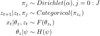
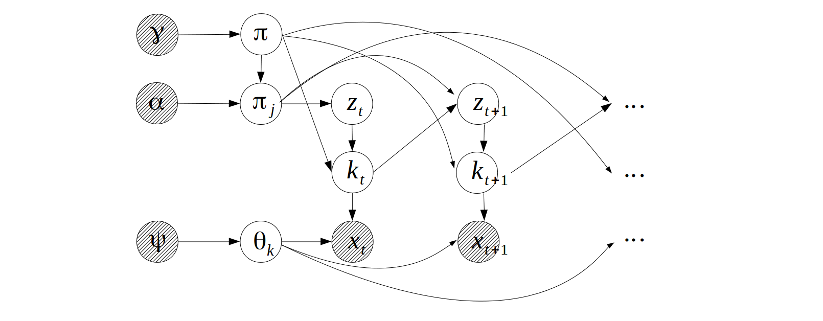
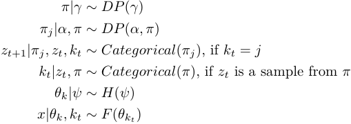
An infinite state hidden Markov model can be represented by a hierarchical Dirichlet process according to Teh (2005), the graphical model for HDP-HMM is:
The CPDs are:
Like the one described in Hierarchical Mixture Models, bbricks provides an object of type "HDP" to encode such structures.
For demo purpose I'll use the simple single-move sampling method discussed in Robert et al (1993), Frühwirth-Schnatter (2006) to learn the posterior distributions of the model parameters. See Van Gael et al (2008) for a more efficient implementation.
The R code is:
## Learn HDP-HMM posteriors using single-move sampling

library(bbricks)

source("Programs/Codes/Bayesian Nonparametrics/Dirichlet_Process.r")
## load some hidden markov data
## see ?hmmData for details
data(hmmData)
x <- hmmData$x
Nsegs <- hmmData$Nsegs
breaks <- hmmData$breaks
## Step1: Initialization------------------------------------------
transitionObj <- HDP(gamma = list(gamma=1,alpha=1,j=1,H0aF="GaussianNIW",parH0=list(m=c(0,0),k=0.001,v=3,S=diag(2))))
## place holder for the sampled hidden states
zk <- matrix(0L,ncol = 2,nrow = nrow(x))
## observation sufficient statistics
ssx <- sufficientStatistics(obj = GaussianNIW(),x=x,foreach = TRUE)
## sample k from p(k|gamma,x)
samplePi <- function(x,zkAfter){
    ## allK <- which(transitionObj$Z$Z1$gamma$nk>0)
    allK <- which(transitionObj$Z$Z1$gamma$nk>0) #all possible k
    if(length(allK)==0) return(transitionObj$Z$Z1$gamma$newLabel)
    ## p(k|pi) p(x|k) p(k_{2}|k)
    logp <- dPosteriorPredictive(transitionObj$Z$Z1,x=allK,LOG = TRUE) +
        vapply(allK,function(k){
            dPosteriorPredictive(transitionObj$X[[k]],x=x,LOG = TRUE)+
            dPosteriorPredictive(obj = transitionObj,z=zkAfter[1],k=zkAfter[2],j=k,LOG = FALSE)
        },FUN.VALUE = numeric(1))

    logp <- exp(logp-max(logp))
    allK[sample.int(length(allK),size = 1,prob = logp)]
}
## sample z and k from p(z,k|gamma,alpha,x)
sampleZK <- function(kBefore,zkAfter,x){
    ## p(z,k | k_{t-1}) p(x|k)
    probs <- dAllIndicators(obj = transitionObj,j=kBefore,x=x)
    ##
    allK <- unique(probs$k)

    ## p(k_{t+1} | k)
    p <- vapply(allK,function(k){
        if(k==transitionObj$Z$Z1$gamma$newLabel)
            dPosteriorPredictive(obj = transitionObj$Z$Z1,x=zkAfter[2],LOG = FALSE)
        else
            dPosteriorPredictive(obj = transitionObj,z=zkAfter[1],k=zkAfter[2],j=k,LOG = FALSE)
    },FUN.VALUE = numeric(1))
    idx <- sample.int(nrow(probs),size = 1,prob = p[match(probs$k,allK)]*probs$p)
    c(z=probs$z[idx],k=probs$k[idx])
}
## initialize states with forward assignment
for(i in 1L:Nsegs){
    segStart <- breaks[i]+1L
    segEnd <- breaks[i+1]
    for(j in segStart:segEnd){
        if(j==segStart){
            k <- rPosteriorPredictive(obj = transitionObj$Z$Z1,n=1)
            ## update initial and observation
            posterior(obj = transitionObj,ss=ssx[[j]],ss1=k,ss2=1L,j=k)
            zk[j,2] <- k
        }else{
            ## sample from the j(or k) th DP
            zk1 <- rPosteriorPredictive(obj = transitionObj,n=1,j=zk[j-1,2],x=x[j,,drop=FALSE])
            ## update transition and observation
            posterior(obj = transitionObj,ss = ssx[[j]],ss1=zk1[2],ss2=zk1[1],j=zk[j-1,2])
            ## write to book
            zk[j,] <- zk1
        }
    }
}
## Step2: main Gibbs loop---------------------------------------------
maxit <- 20
it <- 1
pb <- txtProgressBar(min = 0,max = maxit,style = 3)
while(it<=maxit){
    ## for all segments
    for(i in 1L:Nsegs){
        segStart <- breaks[i]+1L
        segEnd <- breaks[i+1]
        for(j in segStart:segEnd){
            ## discard previous z
            if(j==segStart){
                ## discard 1 obs 1 initial and 1 transition
                posteriorDiscard(obj = transitionObj,ss=ssx[[j]],ss1=zk[j,2],ss2=1L,j=zk[j,2])
                posteriorDiscard(obj = transitionObj,ss=NULL, ss1=zk[j+1,2],ss2=zk[j+1,1],j=zk[j,2])
                ## sample new initial k
                k <- samplePi(x=x[j,,drop=FALSE],zkAfter = zk[j+1,,drop=FALSE])
                ## update prior with newly sampled k
                posterior(obj = transitionObj,ss=ssx[[j]],ss1=k,ss2=1L,j=k)
                posterior(obj = transitionObj,ss=NULL, ss1=zk[j+1,2],ss2=zk[j+1,1],j=k)
                ## write to book
                zk[j,2] <- k
            }else if(j==segEnd){
                ## discard 1 obs and 1 transition
                posteriorDiscard(obj = transitionObj,ss=ssx[[j]],ss1=zk[j,2],ss2=zk[j,1],j=zk[j-1,2])
                ## sample new z k
                zk1 <- rPosteriorPredictive(obj = transitionObj,n=1,x=x[j,,drop=FALSE],j=zk[j-1,2])
                ## update prior with newly sampled z
                posterior(obj = transitionObj,ss=ssx[[j]],ss1=zk1[2],ss2=zk1[1],j=zk[j-1,2])
                ## write to book
                zk[j,] <- zk1
            }else{
                ## discard 2 transitions and 1 obs
                posteriorDiscard(obj = transitionObj,ss=ssx[[j]],ss1=zk[j,2],ss2=zk[j,1],j=zk[j-1,2])
                posteriorDiscard(obj = transitionObj,ss=NULL, ss1=zk[j+1,2],ss2=zk[j+1,1],j=zk[j,2])
                ## sample new z k
                zk1 <- sampleZK(kBefore = zk[j-1,2],zkAfter = zk[j+1,],x=x[j,,drop=FALSE])
                ## update prior with newly sampled z k
                posterior(obj = transitionObj,ss=ssx[[j]],ss1=zk1[2],ss2=zk1[1],j=zk[j-1,2])
                posterior(obj = transitionObj,ss=NULL, ss1=zk[j+1,2],ss2=zk[j+1,1],j=zk1[2])
                ## write to book
                zk[j,] <- zk1
            }
        }
    }
    it <- it+1
    setTxtProgressBar(pb,it)
}
allK <- which(transitionObj$Z$Z1$gamma$nk>0)
## print the MAP estimates of the state transitions
for(k in allK) print(vapply(split(MAP(transitionObj$Z$Z2[[k]]),f=transitionObj$Z$Z12map[[k]]),sum,numeric(1)))
## print the MAP estimates of the observation parameters
for(k in allK) print(MAP(transitionObj$X[[k]]))
## print the MAP esitmate of the initial state distribution
round(MAP(transitionObj$Z$Z1)[allK],2)
Andrieu, Christophe, et al. "An introduction to MCMC for machine learning." Machine learning 50.1-2 (2003): 5-43.
Johnson, Valen E., and James H. Albert. Ordinal data modeling. Springer Science & Business Media, 2006.
Hoff, Peter D. A first course in Bayesian statistical methods. Vol. 580. New York: Springer, 2009.
Li, Yuelin, Elizabeth Schofield, and Mithat Gönen. "A tutorial on Dirichlet process mixture modeling." Journal of Mathematical Psychology 91 (2019): 128-144.
MARolA, K. V., JT KBNT, and J. M. Bibly. Multivariate analysis. AcadeInic Press, Londres, 1979.
McLachlan, Geoffrey J., and Thriyambakam Krishnan. The EM algorithm and extensions. Vol. 382. John Wiley & Sons, 2007.
Murphy, Kevin P. Machine learning: a probabilistic perspective. MIT press, 2012.
Robert, Christian P., Gilles Celeux, and Jean Diebolt. "Bayesian estimation of hidden Markov chains: A stochastic implementation." Statistics & Probability Letters 16.1 (1993): 77-83.
Frühwirth-Schnatter, Sylvia. Finite mixture and Markov switching models. Springer Science & Business Media, 2006.
Smith, W. B., and R. R. Hocking. Algorithm as 53: Wishart variate generator. Journal of the Royal Statistical Society. Series C (Applied Statistics) 21.3 (1972): 341-345.
Teh, Yee Whye. "Dirichlet Process." (2010): 280-287.
Teh, Yee W., et al. "Sharing clusters among related groups: Hierarchical Dirichlet processes." Advances in neural information processing systems. 2005.
Van Gael, Jurgen, et al. "Beam sampling for the infinite hidden Markov model." Proceedings of the 25th international conference on Machine learning. 2008.
Wishart, John. "The generalized product moment distribution in samples from a normal multivariate population." Biometrika (1928): 32-52.


