Author: Chi Bui
├── README.md               <-- Main README file explaining the project's business case,
│                           methodology, and findings
│
├── notebook                <-- Jupyter Notebooks for exploration and presentation
│   └── exploratory         <-- Unpolished exploratory data analysis (EDA) and modeling notebooks
│
│
├── dataframes              <-- records of all models' performance metrics & propability predictions
│                               on validation set
│
├── reports                 <-- Generated analysis
│   └── report-notebook     <-- Polished final notebook
│   └── presentation.pdf    <-- Non-technical presentation slides
│
│
└── images                  <-- Generated graphics and figures to be used in reporting
(source: Wikipedia)
Pneumonia is an inflammatory condition of the lung primariy affecting the small air sacs known as alveoli in one or both lungs. It can be caused by infection with viruses or bacteria; and identifying the pathogen responsible for Pneumonia could be highly challenging.
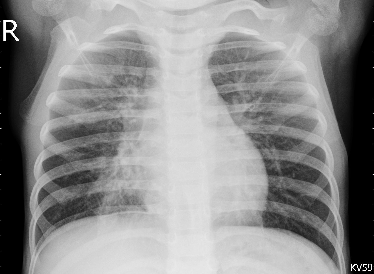
Diagnosis of Pneumonia often starts with medical history and self reported symptoms, followed by a physical exam that usually includes chest auscultation. A chest radiograph would then be recommended if the doctors think the person might have Pneumonia. In adults with normal vital signs and a normal lung examination, the diagnosis is unlikely.
Pneumonia remains a common condition associated with considerable morbidity and mortality - each year it affects approximately 450 million people, and results in about 4 million deaths. Outcome is often improved by early diagnosis, yet the traditional radiograph assessment usually introduces a delay to the diagnosis and treatment. Therefore, fast and reliable computer-aided diagnosis of the disease based on chest X-ray could be a critical step in improving the outcomes for Pneumonia patients.
For this project, I have developed and evaluated various Convolutional Neural Networks that can quickly classify Normal vs. Pneumonia frontal chest radiographs. The implementation of these models could help alert doctors and radiologists of potential abnormal pulmonary patterns, and expedite the diagnosis.
The dataset was collected from Guangzhou Women and Children’s Medical Center (Guangzhou, China) pediatric patients of one to five years old.
The dataset is available on:
The diagnoses for the images were then graded by two expert physicians, and checked by a third expert before being cleared for training the AI system.
The dataset is divided into 2 directories:
- train
- test
Within each directory, there're 2 sub-directories:
- NORMAL
- PNEUMONIA
and the labels for the images are the names of the corresponding directories they're located in.
chest_xray
    │
    ├── test
    │   ├── NORMAL
    │   │   └── image_01.jpeg
    │   └── PNEUMONIA
    │       └── image_02.jpeg
    └── train
        ├── NORMAL
        │   └── image_01.jpeg
        └── PNEUMONIA
            └── image_02.jpeg
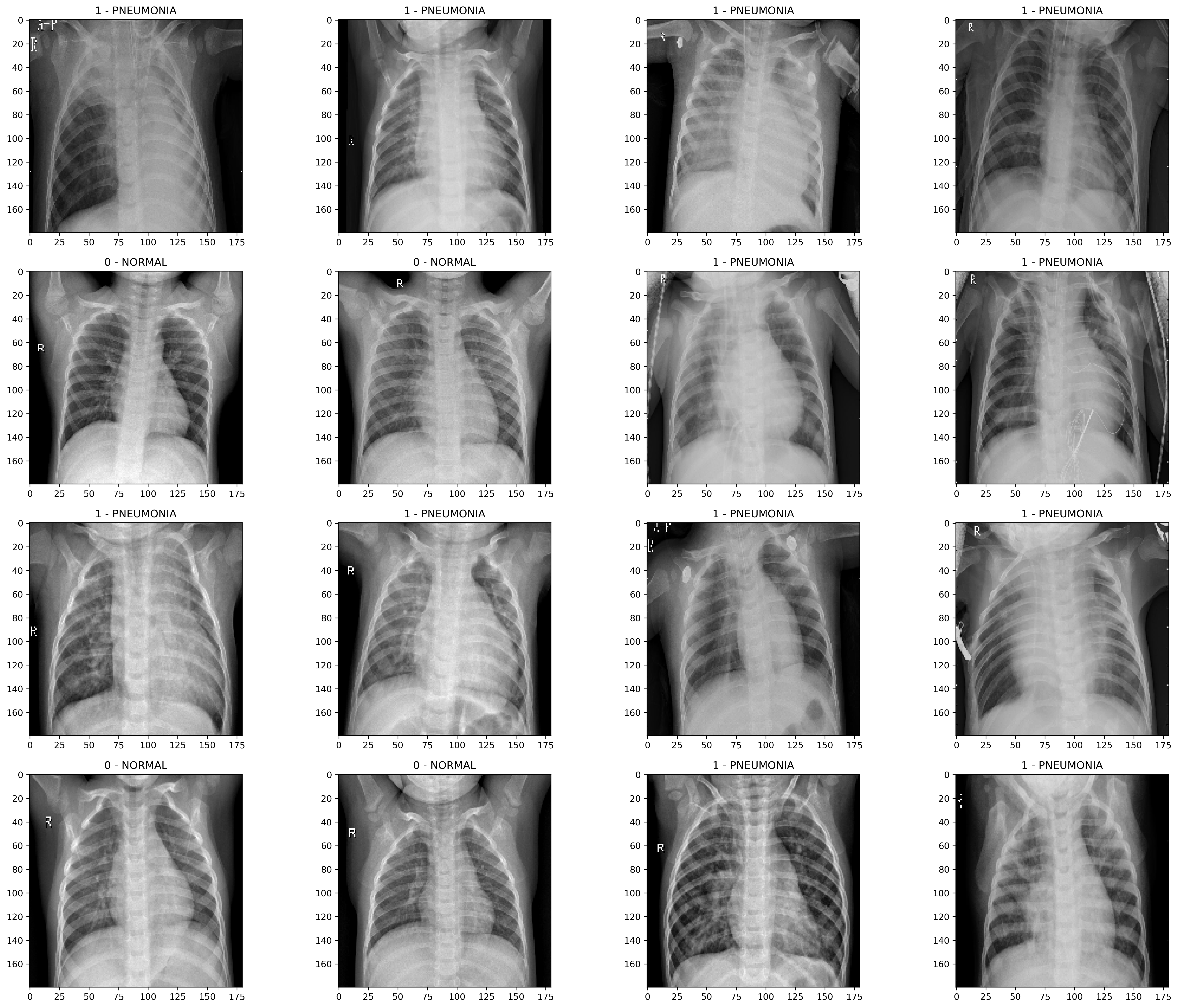
Although a printout of these images' shapes indicate that they're composed of 3 channels (RGB), a comparison of 3 layers' numerical values are exactly the same.
For this reason, moving forward, I would set ImageDataGenerator()'s color_mode to grayscale to downsize the dataset, while still retaining the same amount of information.
In order to easily analyze this dataset's class composition and evaluate its balancedness, I would create a dataframe with 2 columns:
- 1st column: name of the image file - called
image - 2nd column: label for that image - called
label
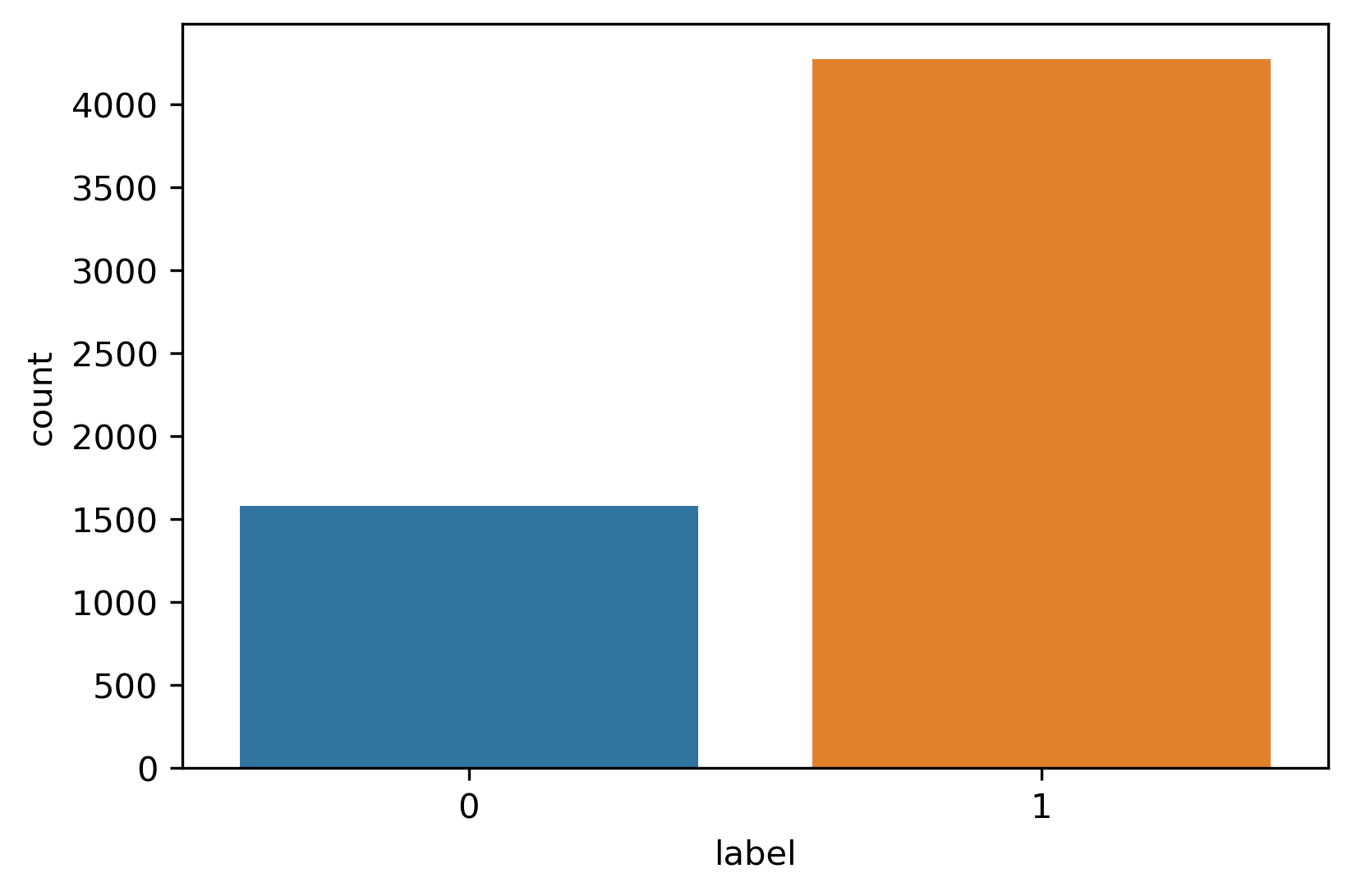
There are 5232 images in the training set (with an approximately 3:1 class ratio), and only 624 in test set (with less than a 2:1 ratio).
In addition, due to a potential "mislabeling" issue in the test data (which has been raised about this dataset in various different platforms), I'm going to concatenate both sets together and re-split them into Train/Validation/Test later to ensure data consistency.
After joining, in total we have 5856 images, out of which Pneumonia takes up 72.9%.
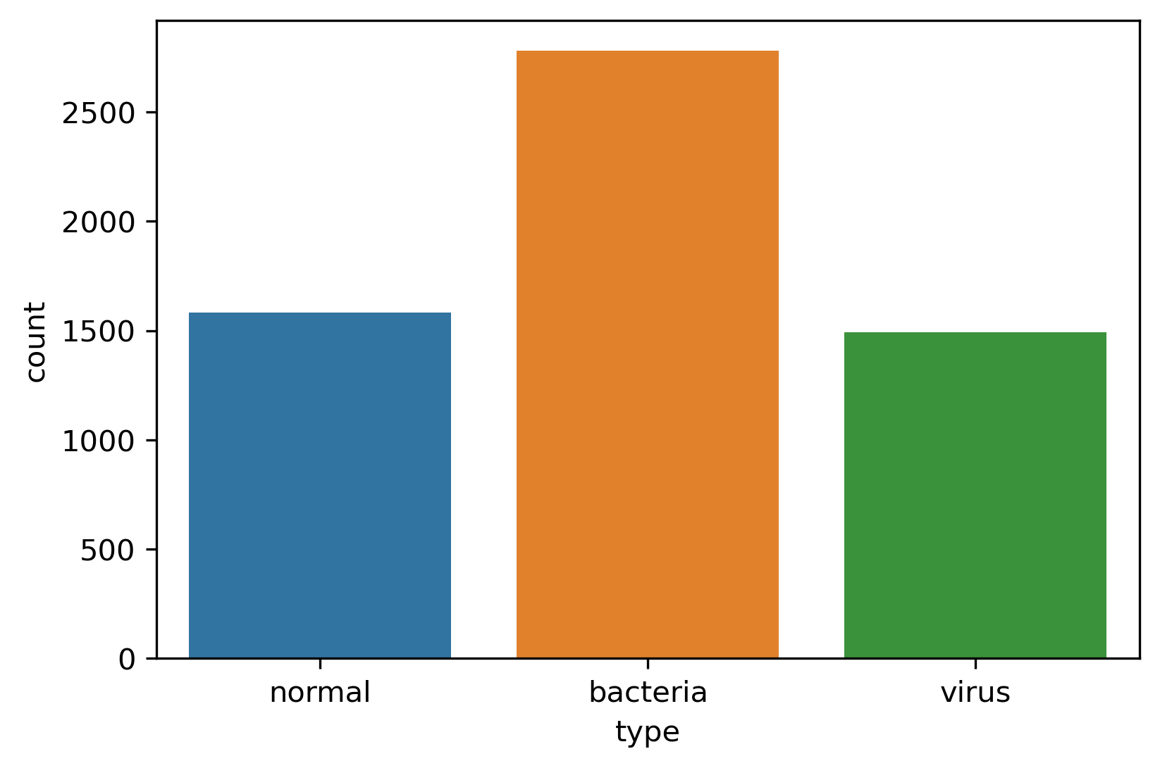
Within the Pneumonia class itself, there are two different types: Bacteria and Virus. These 2 subclasses that usually observed with some distinctive characteristics:
- Bacterial pneumonia typically exhibits a focal lobar consolidation
- whereas Viral pneumonia manifests with a more diffuse ‘‘interstitial’’ pattern in both lungs
These differences would potentially impact the models' capabilities to differentiate the X-ray images; therefore it might be valuable to include this information in the model evaluation. This would not be the main focus of this project, but it would certainly provide some information for us to dig deeper into this topic in the future, and perhaps train models to identify responsible Pneumonia pathogens.
4273 datapoints in our master dataset are categorized as PNEUMONIA, which accounts for roughly 73% of the whole set:
- Roughly 2/3 of the Pneumonia X-ray images are Bacterial Pneumonia
- The other 1/3 are Viral
This means that we're working with a highly imbalanced dataset, and I would need to counter this by assigning class weights or incorporating some image augmentation methods later. Our models are also going to be less exposed to Viral Pneumonia, and might struggle with these X-ray more than with Bacterial.
Using sklearn's train_test_split, I then split the master dataframe into 3 smaller sets:
- Training (
train_df) - used for fitting models directly - Valuation (
val_df) - used for model tuning during iterations - Test (
test_df) - used for final model evaluation
My models would be trained mainly on the training set, and also exposed to the valuation set but only for the purpose of evaluating the model on a small unseen dataset.
Final model would then be evaluated on the Test set.
(Source: Hands-on Machine Learning with Scikit-Learn, Keras & TensorFlow - Aurelien Geron)
Convolutional Neural Networks have proved to be highly accurate with Image Recognition tasks, partly due to its resemblence of nature.
David H. Hubel and Torsten Wiesel's experiments on cats (in 1958 and 1959), and on monkeys a few years later has led them to discover some crucial insights into the structure of the visual cortex:
- They found out that many neurons in the visual cortex have a small local receptive field (which means they only react to visual stimuli in a limited region of the visual field). The receptive fields of different neurons may overlap, they work together to create the whole visual field.
- In addition, some neurons react only to images of horizontal lines, while others react to lines with other orientations (two neurons with the same receptive field might detect different line orientations).
These studies of the visual cortex had inspired the neocognitron in the 80s, which gradually evolved into modern convolutional neural networks.
-
Convolutional Layers Convolutional Layer is the building block of CNN. Neurons in the 1st convolutional layer are only connected to pixels in their receptive field. Then each neuron in the 2nd convolutional layer is only connected to neurons within their receptive field in the 1st layer, and so on. This hierarchical structure resembles real-world images
-
Pooling Layers The goal of pooling layer is to subsample the input image inorder to reduce computational load, memory usage, and number of parameters.
Since the objective of this project is to create computer-aided detection model that helps speed up the diagnosis of Pneumonia, and the Accuracy for a highly imbalanced dataset could be skewed, prioritizing a high Recall score and reducing the number of False Negatives (actual Pneumonia cases that are classified as Normal) would be my main goal as I go through model iterations.
As this is an imbalanced dataset with the majority being Pneumonia, a model that predicts everything as Pneumonia would have approx. 73% accuracy (depending on the class ratio of the evaluation set this might vary more or less). If not corrected, models trained on imbalanced dataset would have the tendency to predict more of the abundant class (which is 1-PNEUMONIA in this case).
From the business stand point, a model that predicts more Pneumonia is not entirely bad, because it would reduce the risk of mis-classifying PNEUMONIA cases as NORMAL. Although that could cause some inconveniencies to some people, it would helps ensure higher chance of catching the disease early. However, not correcting class imbalance could also lead to models not learning to differentiate images of the 2 classes efficiently and not picking up the important features of the images.
Please refer to the final notebook for more details on the first 3 models (baseline, cnn_2, and cnn_3) that I have trained prior to the final model cnn_4 using Transfer Learning with ResNet50.
ResNet or Residual Network is one of the most powerful deep neural networks: it helped Kaiming He et al. win the ILSVRC in 2015. The winning variant used an extremely deep CNN with 152 layers; but I'm just going to use ResNet50, which is composed of 48 Convolutional Layers, 1 Max Pool, and 1 Average Pool layer.
Deeper networks can usually represent more complex features, therefore increase the model robustness and performance. However, research has found that stacking up more and more layers creates accuracy degradation (accuracy values start to saturate or abruptly decrease), which is caused by the vanishing gradient effect.
As the number of layers increases, the gradient gets smaller and smaller as it reaches the end layers of the network. Therefore, the weights of the initial layers will either update very slowly or remains the same, which means the initial layers of the network won’t learn effectively.
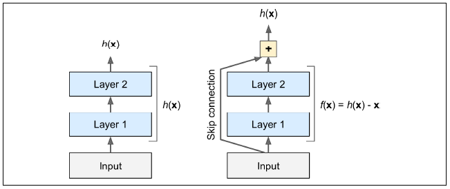
The key to being able to train deep network effectively is skip connection or shortcut connection between the layers:
The idea behind it is to add the input feeding into a layer to the output of a layer higher up the stack.
The goal of training a neural network is to make it model a target function h(x). Adding the input x to the output of the network would then force the network to model f(x) = h(x) - x rather than h(x). This helps speed up training considerably and the networks can start making progress even in several layers have not started learning yet.
Pretrained models like ResNet are readily available with a single line of code in the keras.applications package; therefore we don't have to implement them from scratch.
By default, ResNet takes input shape of (224, 224, 3). Therefore even though I used grayscale for my first 3 models, I had to recreate Image Data Generator with color_mode = rgb to match pretrained models' expected input format.
We can load the ResNet50 model that has been pretrained on ImageNet as follows:
resnet = ResNet50(include_top=False,
                  weights='imagenet',
                  input_shape=(INPUT_SHAPE))
We exclude the top layers (the global average pooling layer & the dense output layer) of the network by setting include_top=False.
Then we add our own global average pooling layer based on the output of resnet base model, and finally followed by a dense output layer with 1 unit using the sigmoid activation function.
# APPLY OUR OWN GLOBAL MAXPOOLING BASED ON THE OUTPUT OF resnet
gmp = GlobalAveragePooling2D()(resnet.output)

# ADD FINAL DENSE LAYER
output = Dense(1, activation='sigmoid')(gmp)
Last but not least, to bind everything together, we create the Keras Model:
# BIND ALL
cnn_4 = Model(resnet.input, outputs=output)

# FREEZE THE WEIGHTS OF resnet BASE MODEL
# SO THAT THEY'RE NON-TRAINABLE
for layer in resnet.layers:
    layer.trainable = False
Since the new output layer was initialized randomly, it would make larger errors, which could damage the pretrained weights. Therefore, it's usualy a good idea to freeze the pretrained layers during the first few epochs. That way the new layer has some time to learn some decent weights (validation accuracy in the 70-80% range).
Then we can compile the model:
# USING SGD TO CUSTOMIZE LEARNING RATE
sgd = SGD(lr=0.02, decay=0.01, momentum=0.9)
cnn_4.compile(optimizer=sgd,
              loss='binary_crossentropy',
              metrics=['accuracy', recall, precision])
cnn_4.summary()
Start the beginning of training:
checkpoint_cb = ModelCheckpoint('cnn_4.h5',
                                save_best_only=True,
                                monitor='val_loss',
                                mode='min')
early_stopping_cb = EarlyStopping(patience=3,
                                  restore_best_weights=True,
                                  monitor='val_loss',
                                  mode='min')

EPOCHS = 5

results_4 = cnn_4.fit(resnet_train_generator,
                      validation_data=resnet_val_generator,
                      epochs=EPOCHS,
                      class_weight=class_weight,
                      steps_per_epoch=(resnet_train_generator.n//BATCH_SIZE),
                      validation_steps=(resnet_val_generator.n//BATCH_SIZE),
                      callbacks=[checkpoint_cb, early_stopping_cb])
After 5 epochs, we unfreeze the layers, recompile and continue training. For the second round of training, I reduced learning rate lr to 0.01 to avoid damaging the pretrained weights:
# UNFREEZE resnet LAYERS FOR 2ND ROUND OF TRAINING:
for layer in resnet.layers:
    layer.trainable = True

# REDUCING LEARNING RATE TO 0.01 TO AVOID DAMANGING THE PRETRAINED WEIGHTS
sgd = SGD(lr=0.01, decay=0.001, momentum=0.9)

# RE-COMPILE MODEL AFTER UNFREEZING ALL LAYERS
cnn_4.compile(optimizer=sgd,
              loss='binary_crossentropy',
              metrics=['accuracy', recall, precision])


checkpoint_cb = ModelCheckpoint('cnn_4.h5',
                                save_best_only=True,
                                monitor='val_loss',
                                mode='min')
early_stopping_cb = EarlyStopping(patience=10,
                                  restore_best_weights=True,
                                  monitor='val_loss',
                                  mode='min')


# INCREASING NUMBER OF EPOCHS BACK TO 30
EPOCHS = 30

results_4 = cnn_4.fit(resnet_train_generator,
                      validation_data=resnet_val_generator,
                      epochs=EPOCHS,
                      class_weight=class_weight,
                      steps_per_epoch=(resnet_train_generator.n//BATCH_SIZE),
                      validation_steps=(resnet_val_generator.n//BATCH_SIZE),
                      callbacks=[checkpoint_cb, early_stopping_cb])
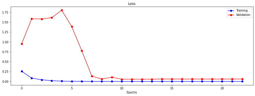
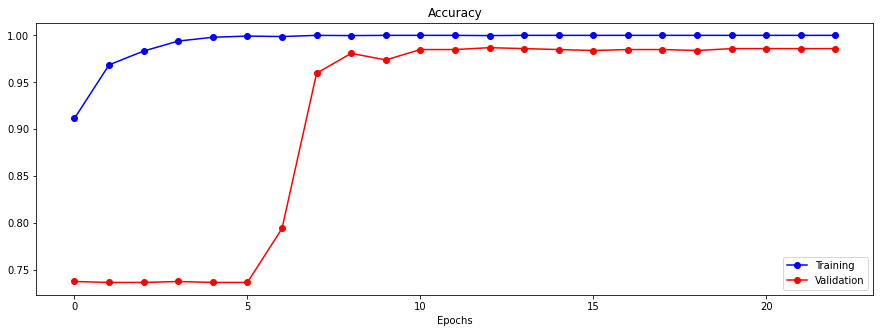
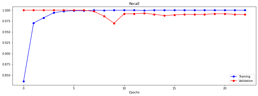
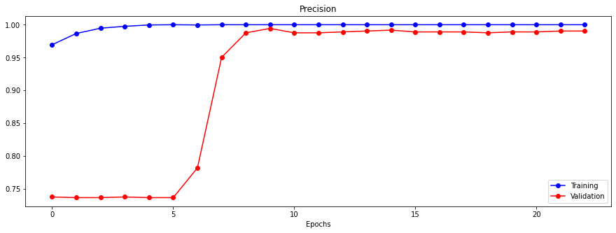
It's actually very interesting to see how the model appeared to be "stuck" at a local optima(?) the first 8 epochs, barely made any progress, and then turned around and increased accuracy by almost 20% from epoch 8 to epoch 9.
| model | loss | accuracy | recall | precision | |
|---|---|---|---|---|---|
| 0 | baseline | 0.0891632 | 0.964859 | 0.974114 | 0.978112 |
| 1 | cnn_2 | 0.113521 | 0.960843 | 0.982289 | 0.965194 |
| 2 | cnn_3 | 0.101416 | 0.968876 | 0.974114 | 0.983494 |
| 3 | cnn_4 | 0.0569717 | 0.986948 | 0.993188 | 0.989145 |
Although all 4 models have very high overall accuracy, cnn_4 has higher Accuracy, Recall and Precision across the board.
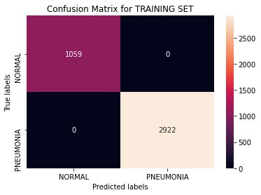
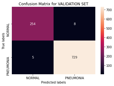
Printouts of the confusion matrices (Training vs. Validation set) shows that there's some overfitting (the model has a 100% accuracy on the training set, and 98.69% on the Validation set). Yet this gap is relatively small.
We can also look at the False Negative cases by 3 previous models that were corrected by cnn_4:
2 out of 4 images have a probability prediction of 0.999. It would be interesting to later see what the model deemed to be discriminative features of these images.
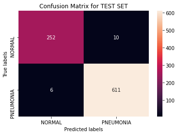
Out of 617 actual Pneumonia X-rays, cnn_4 was able to accurately detect 611, which gives us a very high Recall score of 99.02%. Overall, the model has an Accuracy score of 98.17% on the Test dataset.
Neural Networks are commonly referred to as black-box models because the structure of the networks does not really give us any insights on the structure of the function modeled as well as its relationship with the independent features.
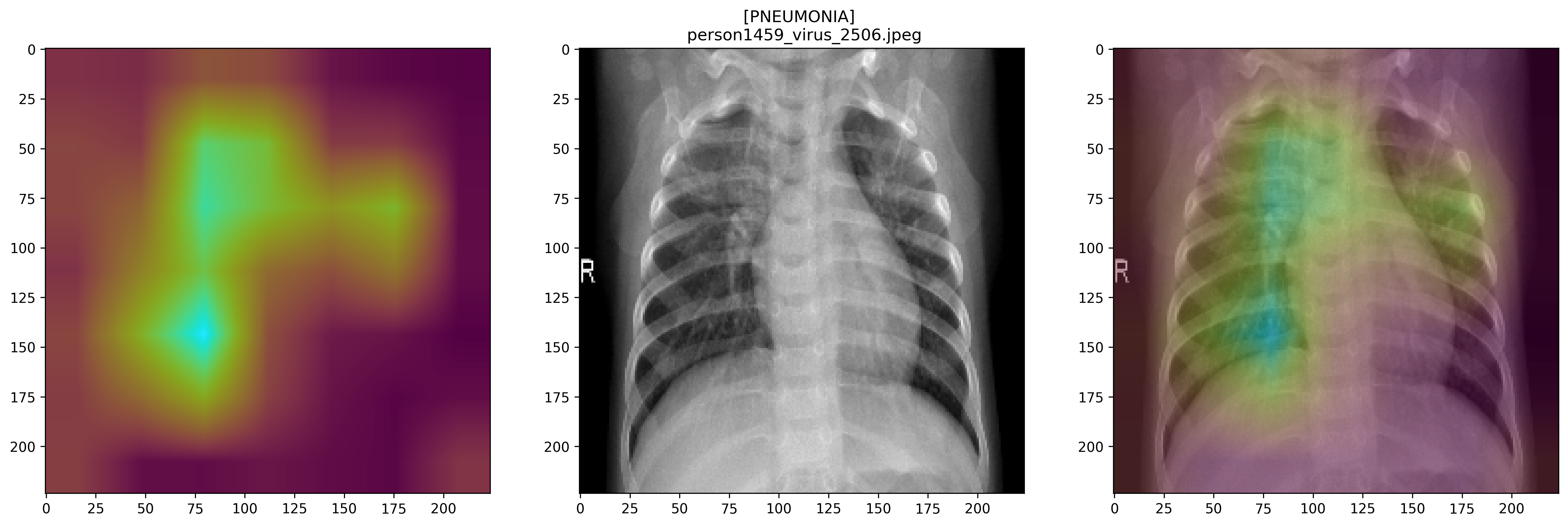
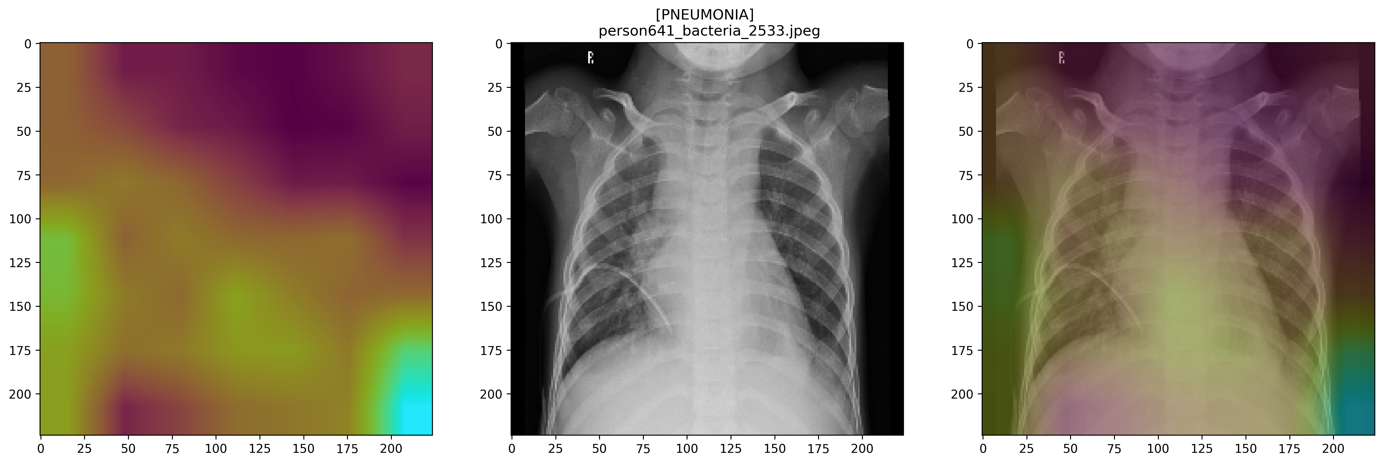
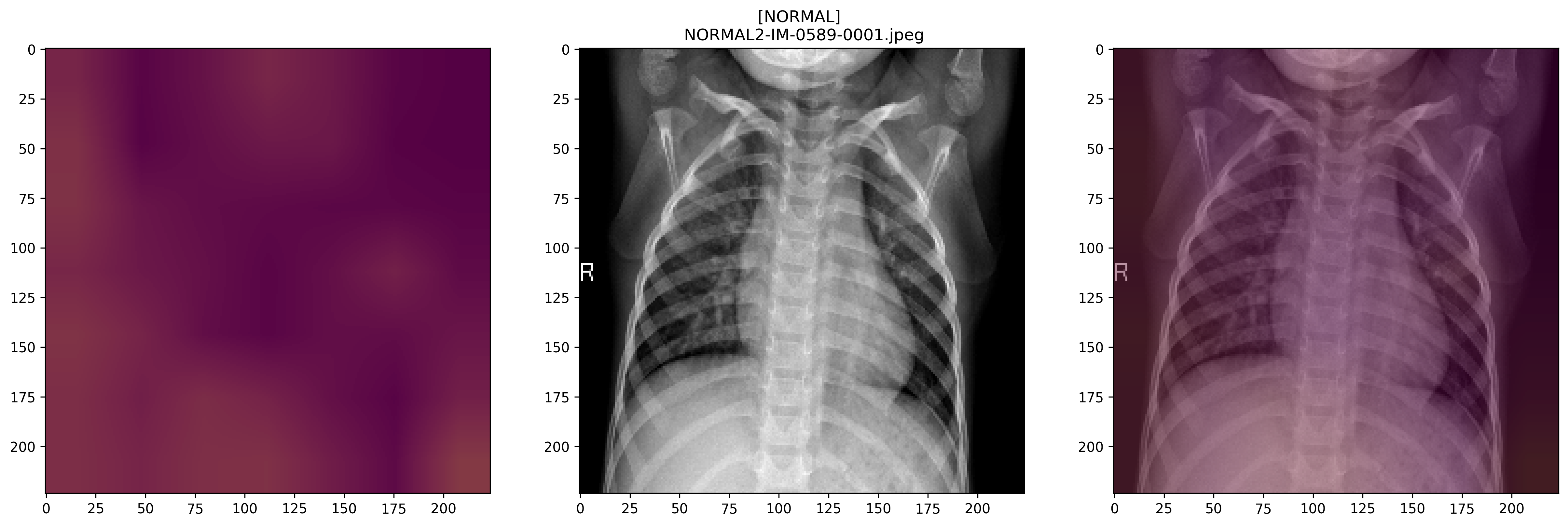
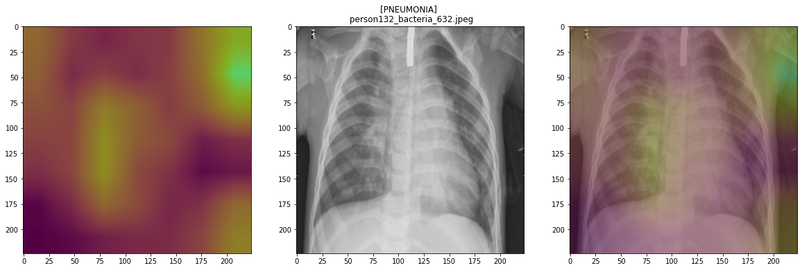
Gradient Class Activation Map (Grad-CAM) for a particular class indicates regions on the images that the CNN used to identify that class. Since this project is a binary classification task, Grad-CAM would hopefully highlight discriminative areas of the X-ray that the models used to differentiate Pneumonia vs. Normal.
For this demonstration, I selected 2 of the 4 Pneumonia X-rays that all 3 previous have failed on, but yet cnn_4 was able to correctly identified with very high probability (0.99):
On this image, Grad-CAM output for this image shows that the model actually used most of the surrounding as the differentiating factor. It does highlight some areas in the chest and in the middle of the spine as well.
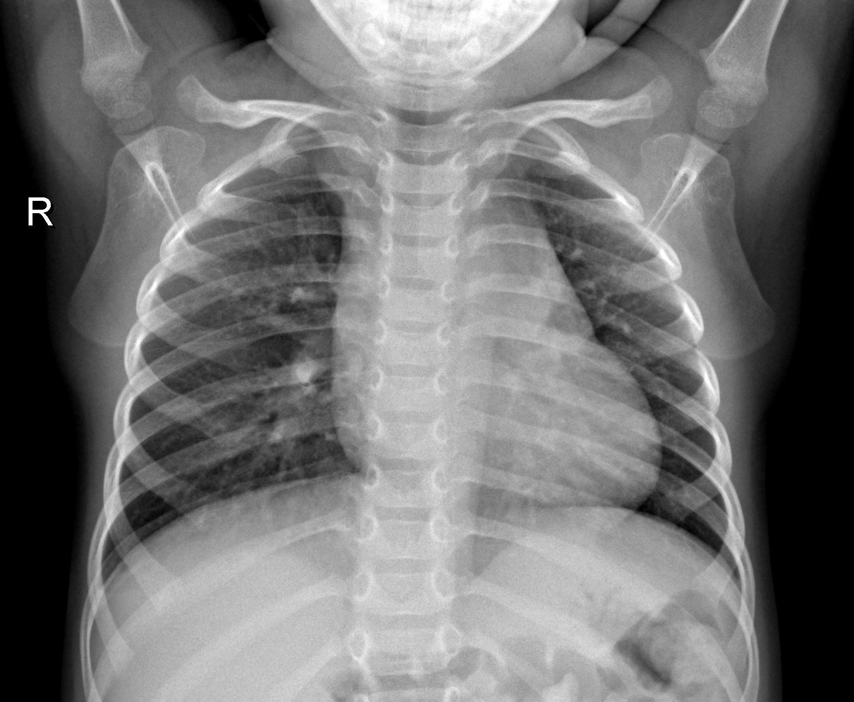
Then I also selected another image in the Normal class with high probability (over 0.9):
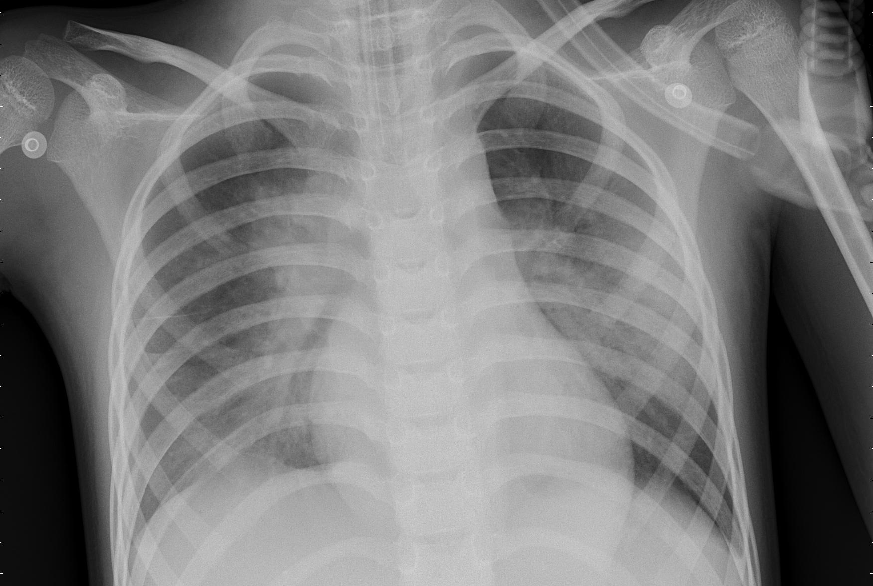
and 1 more Pneumonia X-ray with high probability (over 0.9)
Again, the model seemed to have highlighted the lungs area, and some surrounding like the underarm areas.
Although the final model has achieved very high performance scores across the board (Accuracy, Recall, as well as Precision), Grad-CAM has showed us that the model is still picking up some regions outside the lungs area to identify Pneumonia.
Rather than purely pursuing better metric scores, it'd be best to take advantage of experts' domain knowledge, and have these Grad-CAM outputs reviewed by clinicians and radiologists who can provide input on whether or not the model has identified correct/potential regions the chest area that might be indicators of Pneumonia.
In the future I would want to consider incorporating Object Detection/Localization into the models so that the output would not only be whether or not the X-ray exhibit abnormal pulmonary patterns typically observed in Pneumonia, but also the location of the identified patterns. However, this types of tasks usually requires data that have been labeled with bounding boxes or similar Furthermore, there's potential in developing models that can assist in classifying responsible pathogens for Pneumonia.
- Géron, A. (2019). In Hands-on machine learning with Scikit-Learn & TensorFlow: concepts, tools, and techniques to build intelligent systems. O'Reilly Media, Inc.
- https://machinelearningmastery.com/how-to-use-transfer-learning-when-developing-convolutional-neural-network-models/
- https://www.kaggle.com/suniliitb96/tutorial-keras-transfer-learning-with-resnet50
- https://towardsdatascience.com/deep-learning-using-transfer-learning-python-code-for-resnet50-8acdfb3a2d38
- Wikipedia
