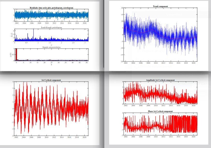
The fSWp models periodical time series considering that the periodicity and trend evolve stochastically according to possibly nonstationary long memory processes. It is estimated by linear state space methods (Kalman Filter).
This repository contains packages of MATLAB functions that can be used to fit various time series with seasonal signals occurring within a geodetic context:
- vertical displacement time series from the Global Navigation Satellite Systems (DTS),
- Non Tidal Atmospheric Loading time series (NTAL),
- hydrological mass loading (HYDL),
- precipitable water vapor (PWV) time series,
- raw GNSS observations from the tenv format
Each folder contains a main. Its name starts always with "sAPplication". Time series corresponding to the model are saved in ".txt format and can be found in each folder.
Steps for running the software:
- In the sAPplication file: change the name of the time series file you want to fit as follows: "structData = readtable(['nameofthefile.txt']);"
- Press run
- Figures and various goodness of fit indicators are output
You will need MATLAB, version 2022a with the optimization toolbox
- For the use of the HYDL toolbox we recommend the following processor and ram: 11th Gen Intel(R) Core(TM) i7-1185G7 @ 3.00GHz 3.00 GH to get optimal results and 32GB of ram
Each time series can be modelled as: Trend + noise + a*cos(\omega t) + a'*sin(\omega t) where a and a' are the amplitudes of the periodical signals with angular frequency \omega and can be deterministic (constant) or stochastic (time-varying)
You will find 7 toolboxes:
- IGS_forfSW_DETERM_TREND_plus_AR1_model1
- NTAL_forfSW_DETERM_TREND_plus_ARMA11_model2
- PWV_Pangea_DETERM_TREND_plus_AR1_model1
- HYDL_forFSW_RW_TREND_model4
- LPAL_forFSW_RW_TREND_model4
- AllDeterministic_model5
- AllDeterministicFracN
They correspond to the following models:
| Model 1 | Model 2 | Model 3 | Model 4 | Model 5 | |
|---|---|---|---|---|---|
| Trend | deterministic | deterministic | local level stochastic | stochastic | deterministic |
| Noise (linear component) | AR(1) | ARMA(1,1) | AR(1) | irrelevant | AR(1) |
| Noise (periodical component) | stochastic fSW | stochastic fSW | stochastic fSW | stochastic fSW | deterministic |
| Example | IGS DTS | NTAL | tenv format | HYDL, LPAL station | xx |
-
For model 1, 2, and 4 we have used the time series from the International GPS Service (IGS) station DRAO (USA), as well as NEAH and LPAL (strong periodical components)
-
For model 3, we have used examples from Wettzell, Germany with in total of 6 GPS stations (WTZA, WTZJ, WTZR, WTZS, WTZZ and WTZL). The observations are in raw format and contain outliers, data gaps, and jumps. A description of the tenv format can be found in the folder under tenv format.txt.
-
All time series are freely available to download for testing purposes under
HYDL:
http://geodesy.unr.edu/NGLStationPages/GlobalStationList
PWV: https://doi.pangaea.de/10.1594/PANGAEA.862525
IGS GPS: http://geodesy.unr.edu/NGLStationPages/GlobalStationList
Additionally, we provide a set of functions to generate fSWp and fractional noise in the folder "SimulationsFN&fSW". The main file is called "sSimulations.m".
Parameters can be changed to generate a fractional noise or a fSWp. They are described in the file "sSimulations.m".
AllDeterministicFracN is a toolbox that allows fitting time series with a linear trend and deterministic periodical components. The residuals are modelled as a fractional noise, please refer to https://link.springer.com/article/10.1007/BF00665755 exemplarily for a definition. This noise is similar to the power law model as used in the software Hector (Hector user manual version 2.0, p29). The toolbox is available for testing purposes. The main is called sApplicationDetermFracN.m
Note:
-
We have chosen time series with yearly and semi-yearly periodical components. Depending on your context, the frequencies can be changed: vPeriod = [365.25] -> for yearly component ; dLambda = (2pi./vPeriod)(1:harm); -> harm=2 for semi- and yearly components
-
Please avoid changing mX in the main file
-
For fitting other time series with similar functional models, you can change the MATLAB files starting with "fgrid_InitConds". Please contact us for support
The following figures are output: Residual diagnostics (periodogram, autocorrelation), original time series with trend, additional noise on the linear component, amplitude and phase of the periodical components, periodical components. They are automatically saved as .pdf in the folder
We provide a file called "diagnostic.m" which output:
- the AIC, the BIC, the likelihood, the Sum2Corr (sum of square of the sample autocorrelation of the residuals), the value of the trend (not relevant for model 3), the uncertainty of the trend (from the AR(1), the usual formulation in geodesy, see references below) and from the KF
Just run the lines from the quantities you wish to output
-
The cases treated in the available toolboxes are described in: .... arXiv to come
-
You will find further information on the fSWp and the theory at: Proietti, T., & Maddanu, F.(2022). Modelling cycles in climate series: The fractional sinusoidal waveform process. Modeling Cycles In Climate Series. Journal of Econometrics. https://doi.org/10.1016/j.jeconom.2022.04.008
-
The model has been further applied to ethane time series at: Maddanu, F., Proietti, T. Trends in atmospheric ethane. Climatic Change 176, 53 (2023). https://doi.org/10.1007/s10584-023-03508-1
-
For geodetic example, please refer to: Davis, J. L., Wernicke, B. P., and Tamisiea, M. E. (2012), On seasonal signals in geodetic time series, J. Geophys. Res., 117, B01403, doi:10.1029/2011JB008690. Klos, A., Bos, M.S. & Bogusz, J. Detecting time-varying seasonal signal in GPS position time series with different noise levels. GPS Solut 22, 21 (2018). https://doi.org/10.1007/s10291-017-0686-6
-
The MATLAB code has been developed by Federico Maddanu, Laboratory AGM UMR8088, CY Cergy Paris Université, 2 Ave. Adolphe Chauvin, Cergy-Pontoise, 95302, France, with the collaboration of Tommaso Proietti, Department of Economics and Finance, Università di Roma “Tor Vergata”, via Columbia 2, Rome, 00133, Italy.
This study is supported by the Deutsche Forschungsgemein- schaft under the project KE2453/2-1
