In the report, I implement the log-linear model from scratch and update algorithm. The overview of the result is listed below. Besides, I made some effort on using bigram to represent features of text and tested its performance.
| Dataset | best accuracy | best F1-score |
|---|---|---|
| 20news--test | 0.82408391 | 0.81800293 |
| SST5-test | 0.4063 | 0.3649 |
The model is written in Python 3.7. While the core part of the model is implemented from scratch, I import some packages for text preprocessing and metrics calculating, such as nltk, sklearn. To avoid unnecessary exceptions while running the model, versions of these packages are listed below:
| Package | Version |
|---|---|
| Python | 3.7.9 |
| pandas | 1.2.4 |
| numpy | 1.19.2 |
| nltk | 3.6.1 |
| scikit-learn | 0.24.1 |
| argparser | 1.4.0 |
| tqdm | 4.59.0 |
Please set the file structure like this:
homework1/
| -- 20news/
| -- train.csv
| -- test.csv
| -- SST5/
| -- sst_train.csv
| -- sst_test.csv
| -- text_classification.py
| -- lemmatization-en.txt
| -- run.sh
| -- tc_bigram.py
I provide a shell script named run.sh, which can be used to activate the model in terminal. In run.sh, it writes:
# for 20newsgroups dataset
python text_classification.py --dataset 20news --n_classes 20
# for SST5 dataset:
# python text_classification.py --dataset SST5 --n_classes 5
If we want to pass more arguments of the model through run.sh file, we can write:
python text_classification.py --dataset dataset --n_classes n_classes --n_features n_features --lr lr --batch_size batch_size --alpha alpha --n_epoches n_epochesThe arguments are described below:
| Argument | Type | Default | Description |
|---|---|---|---|
| dataset | string, "20news" or "SST5" | "20news" | name of dataset |
| n_classes | integer | 20 | number of classes |
| n_features | integer | 10000 | number of features |
| lr | float | 0.01 | value of learning rate |
| batch_size | integer | 200 | size of each batch |
| alpha | float | 0.0001 | value of regularization coefficient |
| n_epoches | integer | 10 | number of epoches |
My model will be tested on two datasets: 20-Newsgroups and SST-5.
20-Newsgroups is a collection of approximately 20,000 newsgroup documents, partitioned (nearly) evenly across 20 different newsgroups. SST-5 is a sentiment classification dataset, which contains 8544 sentences in training set and 2210 in testing set. There are 5 kinds of labels representing different sentiments.
Before feature extraction, the text should be preprocessed to remove noise. Four methods are used in my code.
- Fisrtly, I remove all of the non-alphanumeric characters and punctuation, and transform every letter to its lower case.
- Secondly, I import
nltk.tokenize.word_tokenize()to split documents to tokens. - Thirdly, with the lemmatization list1 provided by Michal Měchura, I accompoish the lemmatization.
- At last, by importing
nltk.corpus.stopwords.words("english"), stop-words are removed from data.
Besides, tokens whose length are less than 3 are dropped.
from nltk.tokenize import word_tokenize
from nltk.corpus import stopwords

def get_lemma_dict():
    with open('lemmatization-en.txt', 'r') as f:
        lines = f.readlines()
        res_dict = {}
        for line in lines:
            lemma, word = line.strip().split()
            res_dict[word] = lemma
    return res_dict

def preprocess_doc(doc):
    # Remove non-alphanumeric chars and unnecessary punctuation
    # transform to lower case
    doc = re.sub(r"[^A-Za-z0-9]", " ", doc).lower()
    # tokenization
    tokens = word_tokenize(doc)

    res = []
    for token in tokens:
        # lemmatization
        t = lemma_dict[token] if token in lemma_dict else token

        # from autocorrect import Speller
        # spelling correction -- too slow
        # spell = Speller()
        # t = spell(t)

        # stop-words, length limit
        if t not in stop_words and len(t) >= 3:
            res.append(t)
    return res

lemma_dict = get_lemma_dict()
stop_words = set(stopwords.words("english"))
To add, real texts written by human beings are quite complicated, with many miss-spellings, slangs, abbreviations and etc. Since 20newsgroups dataset are constructed from e-mail corpus, there are many spelling errors, like "appearance-appearence" . I tried to import autocorrect.Speller() to accomplish speeling correction, but met low efficiency.
I have adopted some assumptions:
- the appearance of each word is independent(unigram)
- the classification of one text is related to the words appearing in itself
Therefore, to represent the features of the text in training data and testing data, I build a vocabulary from the training data in the beginning:
import pandas as pd

data_train = pd.read_csv(fp_train)
data_train["tokens"] = data_train["data"].apply(lambda x: preprocess_doc(x))
data_test["tokens"] = data_test["data"].apply(lambda x: preprocess_doc(x))

vocabulary = data_train.tokens.apply(pd.Series).stack().value_counts().to_dict()
This vocabulary is sorted by the frequency of appearance of words, by means of values_count(). The I choose the top n_features words to be features, and assign an unique id to each of them:
ngram2id = dict()
for i, item in enumerate(vocabulary.items()):
    if i >= args.n_features:
        break
    ngram2id[item[0]] = i
With ngram2id, we can transform the input text into a series of word ids:
def extract_features(tokens):
    features = []
    for token in tokens:
        if token in ngram2id:
            features.append(ngram2id[token])
    return features

data_train["features"] = data_train["tokens"].apply(lambda x: extract_features(x))
data_test["features"] = data_test["tokens"].apply(lambda x: extract_features(x))
Then, the log-linear model will be trained to capture the relationship between features of text and its labels, and try to predict.
Moreover, I have made some effort based on another assumption: the appearance of each word is related to the word before it(bigram). But a big improvement on model performance didn't show up. The details can be seen in the following section 5 Another Try: Bigram.
According to the teaching slide, we define
- Initialize all
$\lambda s$ to be 0 - Iterate until convergence
- Calculate
$\delta = \frac{\partial LL(\vec{\lambda})}{\partial \lambda}$ - Calculate
$\beta_* = {\underset {\beta}{\operatorname {arg,max}}} ,LL(\vec{\lambda}+\beta*\delta)$ - Set
$\vec{\lambda} = \vec{\lambda} + \beta_* *\delta$
- Calculate
To imploment this algorithm, I use n_epoches to control the number of iterations, which set to be 10. Experiment shows after 10 epoches, the output of the model is very close to convergence in most cases. As for lr, which set be a hyperparameter.
I define a class named `LogLinearModel, whose initialization function is like:
class LogLinearModel:
    def __init__(self, n_classes, n_features, lr, alpha):
        self.n_classes = n_classes
        self.n_features = n_features
        self.lr = lr
        self.alpha = alpha
        self.w = [[0.0 for i in range(n_features)] for k in range(n_classes)]
The description of each argument can be found in the section 1.2 shell script. The 2-dimension array LogLinearModel.w corresponds ro LogLinearModel.w are number of classes and number of features.
In the model LogLinearModel, three functions are defined:
def fit(self, samples, labels, batch_size):
    count = 0
    for i_batch in tqdm(range((len(samples) // batch_size + 1))):
        batch_samples = samples[count: count + batch_size]
        batch_labels = labels[count: count + batch_size]
        self.update(batch_samples, batch_labels)
        count += batch_size
    return
LogLinearModel.fit() is used for training. I use mini-batch gradient ascend method as update algorithm, so when training data is thrown into the model, it will be divided into a number of batches.
import numpy as np

def transform(self, samples):
    labels = []
    list_scores = []
    for sample in samples:
        scores = []
        for i_label in range(self.n_classes):
          	# calculate score(x, y)
            # score(x, y) = f_i(x, y) * lambda_(f_i(x, y)), i range from (0, n_features)
            scores.append(sum([self.w[i_label][token] for token in sample]))
        scores = np.array(scores)
        scores = np.exp(scores-scores.max())  # math range error/overflow encounted in exp if not minus max()
        scores /= scores.sum()
        label = np.argmax(scores)
        labels.append(label)
        list_scores.append(scores.tolist())
    return labels, list_scores
LoglinearModel.transform() is used to predict labels and calculate LogLinearModel.w().
def update(self, samples, labels):
    _, list_scores = self.transform(samples)
    gradient = [[0.0 for i in range(self.n_features)] for k in range(self.n_classes)]
    for i_sample, sample in enumerate(samples):
        for i_feature in sample:
            for i_class in range(self.n_classes):
                if i_class == labels[i_sample]:
                    gradient[i_class][i_feature] += 1.0  # empirical counts
                # expected counts and regularization
                gradient[i_class][i_feature] -= (list_scores[i_sample][i_class] + self.alpha * self.w[i_class][i_feature])
    for i_class in range(self.n_classes):
        for i_feature in range(self.n_features):
          	# update lambda
            self.w[i_class][i_feature] += self.lr * gradient[i_class][i_feature]
    return
As for updating LogLinearModel.update() finishes the job.
I write arg_adjustment.py to implement hyperparameter adjustment. It writes:
import os

for dataset in ["20news", "SST5"]:
    n_classes = 20 if dataset == "20news" else 5
    for n_features in [200, 2000, 10000]:
        for lr in [0.001, 0.01]:
            for batch_size in [1, 200, 1000]:
                for alpha in [0, 1e-4, 1e-2, 1e-1]:  # 2*3*2*3*4 = 144 iterations
                    os.system(f'python text_classification.py'
                          f' --dataset {dataset}'
                          f' --n_classes {n_classes}'
                          f' --n_features {n_features}'
                          f' --lr {lr}'
                          f' --batch_size {batch_size}'
                          f' --alpha {alpha}')
The model will run for 72 times on these two datasets, respectively. The specific results of each run can refer to the appendix Appendix: Hyperparameter Adjustment Records
We use accuracy and macro F1-score as evaluation metrics. Using the default set of arguments shown in section 1.2 shell script, the two metrics improve on the whole after every epoch:
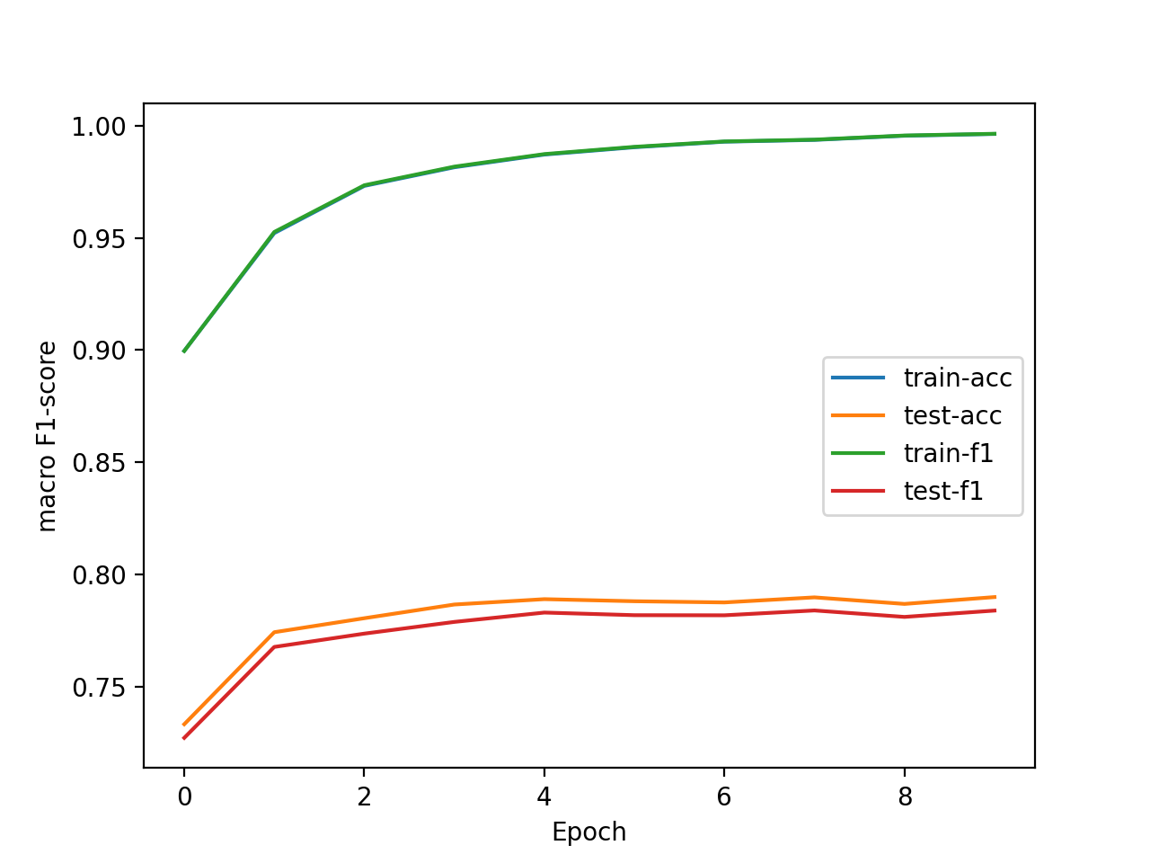 |
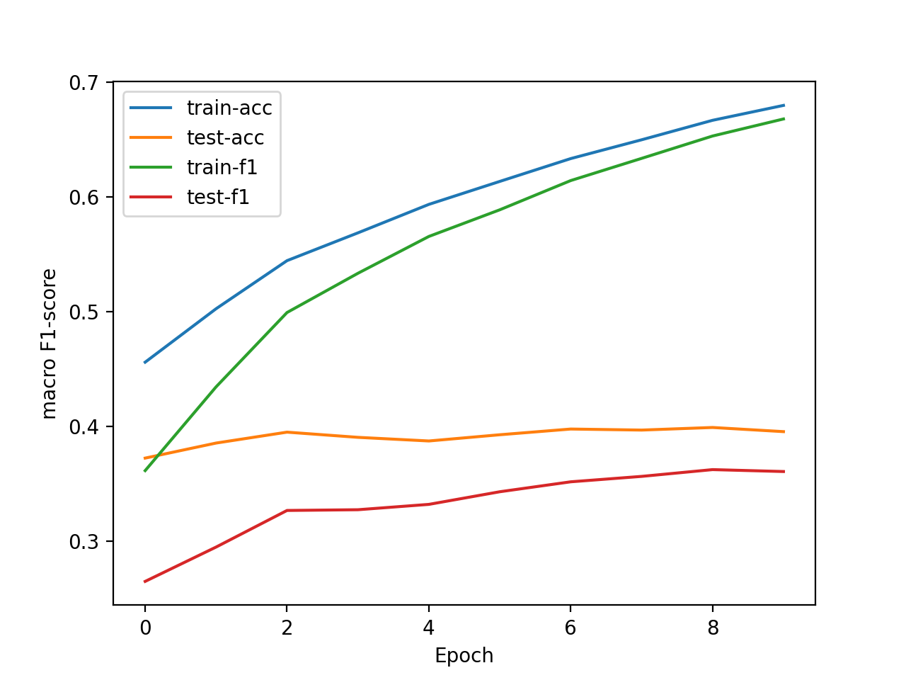 |
|---|
After hyperparameter adjustment described in the last section, the overview of the performance of the model is shown below:
| Best | Worst | |||
|---|---|---|---|---|
| Dataset | accuracy | F1-score | accuracy | F1-score |
| 20news--test | 0.82408391 | 0.81800293 | 0.29221986 | 0.27584847 |
| SST5-test | 0.4063 | 0.3649 | 0.3267 | 0.2400 |
As we can see, the argument sets for the best performance(by macro F1-score) of the model on these two datasets are different :
| alpha | batch_size | lr | n_classes | n_epoches | n_features | test-acc | test-f1 | |
|---|---|---|---|---|---|---|---|---|
| 20news-test | 0.1 | 200 | 0.01 | 20 | 10 | 10000 | 0.82408391 | 0.81800293 |
| SST5-test | 0.01 | 1 | 0.01 | 5 | 10 | 10000 | 0.4 | 0.36491997 |
Moreover, from the appendix, it can be figured out that, compared to regularization coefficient alpha and batch size batch_size, learning rate lr and number of features n_features are more crucial. Models with higher scores mostly set lr to be 0.01 and n_features to be 10000.
To accomplish bigram assunption, the methods for feature representaion and extraction must be rewritten. Take training data as example:
def extract_features_bigram(tokens):
    features = []
    for token in tokens:
        if token in bigram2id:
            features.append(bigram2id[token])
    for i in range(len(tokens)-1):
        if (tokens[i], tokens[i+1]) in bigram2id:
            features.append(bigram2id[(tokens[i], tokens[i+1])])
    return features

data_train["tokens"] = data_train["data"].apply(lambda x: preprocess_doc(x))
data_train["bigram"] = data_train["tokens"].apply(lambda x: [(x[i], x[i + 1]) for i in range(len(x) - 1)])

vocabulary = data_train.tokens.apply(pd.Series).stack().value_counts().to_dict()
vocabulary_bigram = data_train.bigram.apply(pd.Series).stack().value_counts().to_dict()

bigram2id = dict()
for i, item in enumerate(vocabulary.items()):
    if i >= (args.n_features - args.n_bigram):
        break
    bigram2id[item[0]] = i
for i, item in enumerate(vocabulary_bigram.items()):
    if i >= args.n_bigram:
        break
    bigram2id[item[0]] = (i + args.n_features - args.n_bigram)

data_train["features_bigram"] = (data_train["tokens"] + data_train["bigram"]).apply(lambda x: extract_features_bigram(x))
I use n_bigram to control the number of bigram features, the default is 1000. But I didn't see a big improvement. The table below is the performance of bigram model tested on SST5 dataset. Other arguments are set to default.
| n_bigram | acc | f1 |
|---|---|---|
| 0 | 0.39864253 | 0.36121948 |
| 100 | 0.39547511 | 0.36572866 |
| 500 | 0.39683258 | 0.36226996 |
| 1000 | 0.39547511 | 0.36454927 |
| 5000 | 0.4 | 0.36664749 |
| 10000 | 0.24072398 | 0.23719429 |
The bigram model is written in the file tc_bigram.py.
After every run of the model, arguments and the performance will be exported to a .csv file as a log file, which can be found in the folder /log_file. The .csv file is named in the format like: "{args.alpha}-{args.batch_size}-{args.dataset}-{args.lr}-{args.n_classes}-{args.n_epoches}-{args.n_features}.csv".
Tables in the appendix are sorted by the test-f1, from the largest to smallest.
| alpha | batch_size | lr | n_features | test-acc | test-f1 |
|---|---|---|---|---|---|
| 0.1 | 200 | 0.01 | 10000 | 0.82408391 | 0.81800293 |
| 0.1 | 1 | 0.01 | 10000 | 0.82355284 | 0.81776171 |
| 0.01 | 200 | 0.01 | 10000 | 0.81452469 | 0.80904868 |
| 0.01 | 1000 | 0.01 | 10000 | 0.81479023 | 0.80869562 |
| 0.01 | 1 | 0.01 | 10000 | 0.81253319 | 0.80609501 |
| 0.1 | 1 | 0.001 | 10000 | 0.81253319 | 0.80567043 |
| 0.1 | 200 | 0.001 | 10000 | 0.81279873 | 0.80566612 |
| 0.1 | 1000 | 0.001 | 10000 | 0.81040892 | 0.80331566 |
| 0.01 | 1 | 0.001 | 10000 | 0.7952735 | 0.78855116 |
| 0.0001 | 1 | 0.01 | 10000 | 0.7940786 | 0.7884061 |
| 0.01 | 200 | 0.001 | 10000 | 0.79474243 | 0.78795747 |
| 0 | 200 | 0.01 | 10000 | 0.7924854 | 0.78668048 |
| 0.01 | 1000 | 0.001 | 10000 | 0.79261816 | 0.78642263 |
| 0.0001 | 200 | 0.01 | 10000 | 0.79036113 | 0.78430117 |
| 0 | 1 | 0.01 | 10000 | 0.78836962 | 0.78202463 |
| 0 | 1000 | 0.001 | 10000 | 0.78783856 | 0.78131021 |
| 0.0001 | 200 | 0.001 | 10000 | 0.78730749 | 0.78067729 |
| 0.0001 | 1000 | 0.001 | 10000 | 0.78690919 | 0.780207 |
| 0.0001 | 1000 | 0.01 | 10000 | 0.78558152 | 0.77989881 |
| 0 | 1 | 0.001 | 10000 | 0.78624535 | 0.77984117 |
| 0 | 200 | 0.001 | 10000 | 0.78624535 | 0.77954893 |
| 0.0001 | 1 | 0.001 | 10000 | 0.78412108 | 0.77754276 |
| 0 | 1000 | 0.01 | 10000 | 0.78027084 | 0.77445178 |
| 0.1 | 1 | 0.001 | 2000 | 0.76075412 | 0.75391821 |
| 0.1 | 200 | 0.001 | 2000 | 0.75955921 | 0.75284854 |
| 0.1 | 1000 | 0.001 | 2000 | 0.75690388 | 0.75037438 |
| 0.01 | 1 | 0.01 | 2000 | 0.75398301 | 0.7475813 |
| 0.1 | 1 | 0.01 | 2000 | 0.75331917 | 0.7463599 |
| 0.01 | 200 | 0.01 | 2000 | 0.7507966 | 0.74601913 |
| 0.01 | 1000 | 0.01 | 2000 | 0.75 | 0.74372128 |
| 0.01 | 1000 | 0.001 | 2000 | 0.74707913 | 0.74011531 |
| 0.01 | 200 | 0.001 | 2000 | 0.74614976 | 0.73927144 |
| 0.01 | 1 | 0.001 | 2000 | 0.74548593 | 0.73892474 |
| 0 | 200 | 0.01 | 2000 | 0.74336166 | 0.73620319 |
| 0 | 1000 | 0.01 | 2000 | 0.74190122 | 0.73587526 |
| 0 | 1 | 0.01 | 2000 | 0.74176845 | 0.73558958 |
| 0.0001 | 1 | 0.01 | 2000 | 0.74083909 | 0.73436695 |
| 0.1 | 200 | 0.01 | 2000 | 0.73990972 | 0.73411062 |
| 0.0001 | 200 | 0.01 | 2000 | 0.73924588 | 0.73378538 |
| 0.0001 | 1000 | 0.001 | 2000 | 0.74057355 | 0.73313502 |
| 0 | 1000 | 0.001 | 2000 | 0.73937865 | 0.73222931 |
| 0 | 200 | 0.001 | 2000 | 0.73818375 | 0.73129025 |
| 0.0001 | 1 | 0.001 | 2000 | 0.73698885 | 0.73021353 |
| 0.0001 | 200 | 0.001 | 2000 | 0.73698885 | 0.72973879 |
| 0 | 1 | 0.001 | 2000 | 0.73605948 | 0.7294352 |
| 0.0001 | 1000 | 0.01 | 2000 | 0.73061604 | 0.72423502 |
| 0.1 | 1000 | 0.01 | 10000 | 0.72012746 | 0.70094982 |
| 0.1 | 1000 | 0.01 | 2000 | 0.62267658 | 0.60419281 |
| 0.0001 | 200 | 0.001 | 200 | 0.46335635 | 0.45556383 |
| 0 | 200 | 0.001 | 200 | 0.46149761 | 0.45396552 |
| 0.01 | 200 | 0.001 | 200 | 0.46282528 | 0.45358646 |
| 0.01 | 1 | 0.001 | 200 | 0.45977164 | 0.45296375 |
| 0.0001 | 1000 | 0.001 | 200 | 0.45844397 | 0.45280643 |
| 0.01 | 1000 | 0.001 | 200 | 0.45990441 | 0.45077217 |
| 0.0001 | 1 | 0.001 | 200 | 0.45446097 | 0.45068743 |
| 0 | 1 | 0.001 | 200 | 0.45924057 | 0.44881851 |
| 0 | 1000 | 0.001 | 200 | 0.45260223 | 0.44762612 |
| 0.1 | 200 | 0.001 | 200 | 0.4539299 | 0.44642612 |
| 0.1 | 1 | 0.001 | 200 | 0.44941583 | 0.44524978 |
| 0.0001 | 1 | 0.01 | 200 | 0.44888476 | 0.44211997 |
| 0.1 | 1000 | 0.001 | 200 | 0.44822092 | 0.43537902 |
| 0.01 | 1 | 0.01 | 200 | 0.44596389 | 0.43449783 |
| 0 | 1 | 0.01 | 200 | 0.44105151 | 0.43203969 |
| 0 | 200 | 0.01 | 200 | 0.42923526 | 0.42673931 |
| 0.0001 | 200 | 0.01 | 200 | 0.43414764 | 0.42447753 |
| 0.01 | 200 | 0.01 | 200 | 0.42405736 | 0.42260667 |
| 0.1 | 1 | 0.01 | 200 | 0.41463091 | 0.40682391 |
| 0 | 1000 | 0.01 | 200 | 0.42113648 | 0.40363687 |
| 0.0001 | 1000 | 0.01 | 200 | 0.39670738 | 0.38118008 |
| 0.1 | 200 | 0.01 | 200 | 0.36909187 | 0.35333292 |
| 0.01 | 1000 | 0.01 | 200 | 0.35833776 | 0.32731531 |
| 0.1 | 1000 | 0.01 | 200 | 0.29221986 | 0.27584847 |
| alpha | batch_size | lr | n_features | test-acc | test-f1 |
|---|---|---|---|---|---|
| 0.01 | 1 | 0.01 | 10000 | 0.4 | 0.36491997 |
| 0.1 | 200 | 0.01 | 10000 | 0.40633484 | 0.36456635 |
| 0.01 | 1000 | 0.01 | 10000 | 0.39954751 | 0.3637897 |
| 0.0001 | 200 | 0.01 | 10000 | 0.39773756 | 0.36376194 |
| 0 | 200 | 0.01 | 10000 | 0.39411765 | 0.36329669 |
| 0.0001 | 1 | 0.01 | 10000 | 0.39954751 | 0.36240455 |
| 0 | 1000 | 0.01 | 10000 | 0.39457014 | 0.36211776 |
| 0.0001 | 1000 | 0.01 | 10000 | 0.39728507 | 0.36075109 |
| 0.01 | 200 | 0.01 | 10000 | 0.39954751 | 0.36036524 |
| 0.1 | 1 | 0.01 | 10000 | 0.39954751 | 0.36030246 |
| 0 | 1 | 0.01 | 10000 | 0.39728507 | 0.36028309 |
| 0.1 | 1000 | 0.01 | 10000 | 0.40090498 | 0.36020449 |
| 0.01 | 1000 | 0.01 | 2000 | 0.39638009 | 0.35806123 |
| 0.0001 | 200 | 0.01 | 2000 | 0.39230769 | 0.3574116 |
| 0 | 1 | 0.01 | 2000 | 0.39095023 | 0.35676707 |
| 0.1 | 200 | 0.01 | 2000 | 0.39864253 | 0.35636279 |
| 0.01 | 200 | 0.01 | 2000 | 0.39049774 | 0.35619864 |
| 0.0001 | 1 | 0.01 | 2000 | 0.38823529 | 0.35507571 |
| 0 | 1000 | 0.01 | 2000 | 0.38461538 | 0.35298986 |
| 0.1 | 1000 | 0.01 | 2000 | 0.39411765 | 0.35293587 |
| 0.0001 | 1000 | 0.01 | 2000 | 0.38733032 | 0.35149885 |
| 0.1 | 1 | 0.01 | 2000 | 0.39728507 | 0.35144022 |
| 0.01 | 1 | 0.01 | 2000 | 0.38687783 | 0.35108053 |
| 0 | 200 | 0.01 | 2000 | 0.3841629 | 0.35063929 |
| 0 | 1000 | 0.01 | 200 | 0.33665158 | 0.30216922 |
| 0.01 | 200 | 0.01 | 200 | 0.33665158 | 0.29901256 |
| 0.0001 | 200 | 0.01 | 200 | 0.33846154 | 0.29811836 |
| 0.01 | 1 | 0.01 | 200 | 0.33800905 | 0.29765012 |
| 0 | 200 | 0.01 | 200 | 0.33348416 | 0.29737553 |
| 0.0001 | 1 | 0.01 | 200 | 0.3321267 | 0.2961226 |
| 0.01 | 1000 | 0.01 | 200 | 0.33257919 | 0.29569543 |
| 0 | 1 | 0.01 | 200 | 0.33574661 | 0.29546731 |
| 0.0001 | 1000 | 0.01 | 200 | 0.33031674 | 0.29313048 |
| 0.1 | 1000 | 0.01 | 200 | 0.34117647 | 0.29300463 |
| 0.1 | 200 | 0.01 | 200 | 0.33574661 | 0.28726162 |
| 0.1 | 1 | 0.01 | 200 | 0.33303167 | 0.28604778 |
| 0.1 | 1000 | 0.001 | 10000 | 0.37692308 | 0.2679967 |
| 0.1 | 200 | 0.001 | 10000 | 0.3760181 | 0.26754004 |
| 0.1 | 1 | 0.001 | 10000 | 0.37556561 | 0.26729358 |
| 0.01 | 200 | 0.001 | 10000 | 0.37058824 | 0.263504 |
| 0.01 | 1 | 0.001 | 10000 | 0.37013575 | 0.2633212 |
| 0.0001 | 1 | 0.001 | 10000 | 0.36968326 | 0.26302194 |
| 0.1 | 200 | 0.001 | 2000 | 0.36968326 | 0.26299253 |
| 0 | 1 | 0.001 | 10000 | 0.36968326 | 0.26297579 |
| 0.01 | 1000 | 0.001 | 10000 | 0.37013575 | 0.26281306 |
| 0.0001 | 200 | 0.001 | 10000 | 0.36923077 | 0.26270562 |
| 0 | 1000 | 0.001 | 10000 | 0.36968326 | 0.26257485 |
| 0 | 200 | 0.001 | 10000 | 0.36968326 | 0.2624948 |
| 0 | 200 | 0.001 | 2000 | 0.36742081 | 0.26226825 |
| 0 | 1 | 0.001 | 2000 | 0.36651584 | 0.26217695 |
| 0.0001 | 1000 | 0.001 | 10000 | 0.36923077 | 0.26179804 |
| 0.01 | 1000 | 0.001 | 2000 | 0.36742081 | 0.26159777 |
| 0.1 | 1 | 0.001 | 2000 | 0.36832579 | 0.26123971 |
| 0.0001 | 1000 | 0.001 | 2000 | 0.36651584 | 0.2610499 |
| 0.0001 | 200 | 0.001 | 2000 | 0.36515837 | 0.26101735 |
| 0.1 | 1000 | 0.001 | 2000 | 0.3678733 | 0.26100517 |
| 0.01 | 200 | 0.001 | 2000 | 0.36606335 | 0.26080921 |
| 0.01 | 1 | 0.001 | 2000 | 0.36606335 | 0.260769 |
| 0.0001 | 1 | 0.001 | 2000 | 0.36515837 | 0.26067891 |
| 0 | 1000 | 0.001 | 2000 | 0.36515837 | 0.26062207 |
| 0 | 1 | 0.001 | 200 | 0.33031674 | 0.24620151 |
| 0.0001 | 1 | 0.001 | 200 | 0.33031674 | 0.24617857 |
| 0 | 200 | 0.001 | 200 | 0.32986425 | 0.24590644 |
| 0.01 | 1 | 0.001 | 200 | 0.32986425 | 0.24588818 |
| 0.01 | 200 | 0.001 | 200 | 0.32986425 | 0.24587618 |
| 0.01 | 1000 | 0.001 | 200 | 0.32941176 | 0.24556958 |
| 0.0001 | 1000 | 0.001 | 200 | 0.32895928 | 0.24532975 |
| 0.0001 | 200 | 0.001 | 200 | 0.32895928 | 0.24496824 |
| 0 | 1000 | 0.001 | 200 | 0.32895928 | 0.24488024 |
| 0.1 | 1 | 0.001 | 200 | 0.32760181 | 0.24126691 |
| 0.1 | 1000 | 0.001 | 200 | 0.32669683 | 0.24072847 |
| 0.1 | 200 | 0.001 | 200 | 0.32669683 | 0.23999604 |