This is a 1D model continuous in space which has the goal to reproduce stop-and-go waves.
Model description is in this article DOI.
Chraibi, M., Tordeux, A., Schadschneider, A. (2016). A Force-Based Model to Reproduce Stop-and-Go Waves in Pedestrian Dynamics. In: Knoop, V., Daamen, W. (eds) Traffic and Granular Flow '15. Springer, Cham. https://doi.org/10.1007/978-3-319-33482-0_22
Model parameters are:
v_0: desired speedtau: reaction timea_0: required space of an agent with zero speeda_v: time constant: velocity-dependency on the speed. Space requirement is defined as:a=a_0 + a_v.v
In the dimensionless version of the model (see article) the above mentioned parameter can be reduced to:
v_0 and a_v.
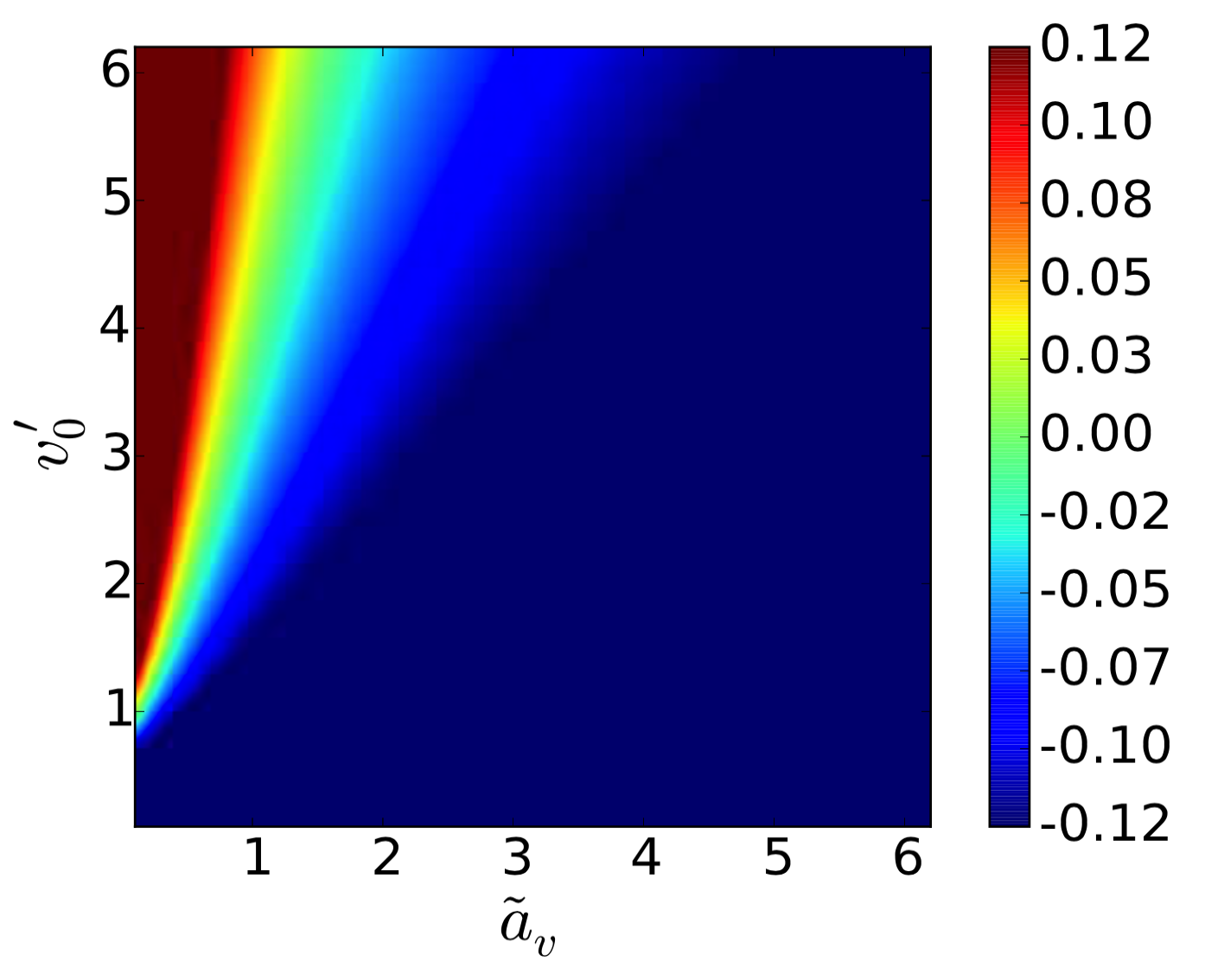
After performing a simplified stability analysis on the model in 1D we find the following relationship:
which indicates for which values of the tuple (v_0,a_v) we can expect having stop-and-go waves.
The following python packages are needed
matplotlibnumpy- (optional)
pandas: for faster loading of the trajectory files.
It recommended to use a virtual environment before installing:
python3 -m venv .venv
source .venv/bin/activate
To install the required libraries run:
pip install -r requirements.txt
python model.py
The following values are used
- Length of the system: 200 m
- Number of pedestrians 133
- Simulation time: 3000 s
v_0=1a_v=0
Note: Run in a separate window tail -f log.txt to display an updated content of the log file.
After successfully running the above script, two files should be produced:
- a trajectory file
- and a log file
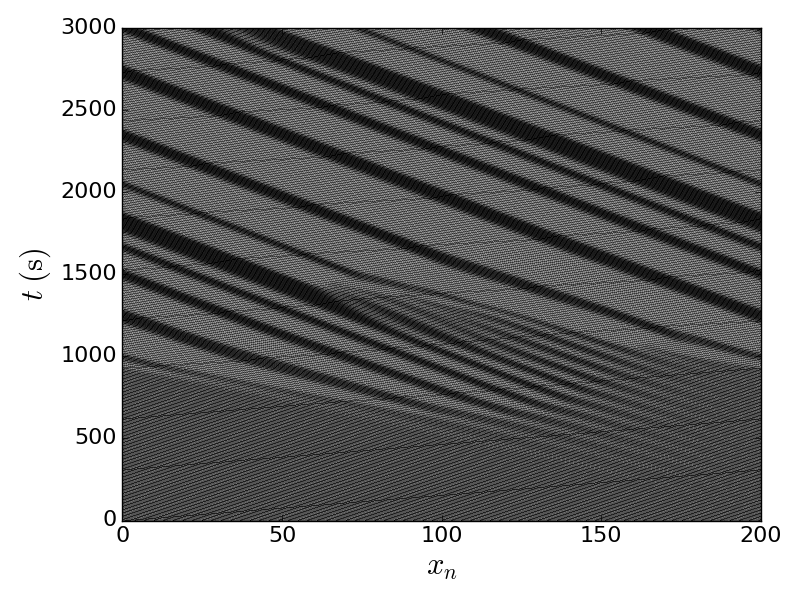
Using the trajectory file we can produce a (x,t) diagram as follows:
python plot-traj.py traj_133_av0.00_v01.00.txt
(Note: the values of the parameter are coded in the name of the file)
The following trajectories are then produced
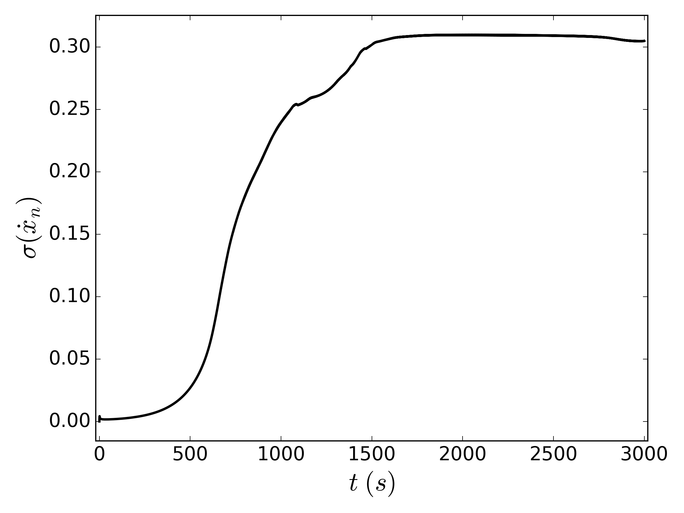
The second file that is produced upon a successful simulation is a log file with some useful speed information (default file name is log.txt).
These can be plotted as well with the following command
python plot_velocity_std.py
which produces this figure


