mkdistmaps

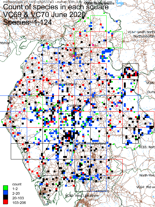
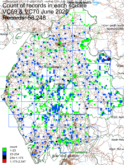
Command line tool to make species distribution maps from species records with grid references. Generated maps are either PNGs on top of a base layer image or geojson files.

Your data can (currently) contain either GB or Irish grid references, but not both. GB grid references start with two letters; Irish grid references start with one letter. The code handles 2, 4, 6, 8 or 10 numbers after the initial letter(s), and also recognises tetrad grid references such as NY12Z and quadrants such as SD11NW.

By default, the generated maps are coloured grouped according to the most recent record in each monad/tetrad or hectad. You can opt to group by the number of records in each square and have an overview map showing how many species are in each square.

You can see example generated geojson maps for lichens in Cumbria at the Cumbria Lichens and Bryophytes website.

Usage: Creating a distribution map PNG image

Ensure you have git and nodejs installed. You will also need your records in CSV format and a base map image.

At a suitable command line prompt:

git clone https://github.com/chriscant/mkdistmaps.git
cd mkdistmaps
npm install

Now get your CSV of records and a basemap image into the new mkdistmaps directory
Make a text file to configure the run eg sample-config.json which you can rename to have a txt extension if that's easier eg vc101-config.txt
Edit your config file to specify your CSV file(s), an output directory and other options
Set the CSV file encoding if need be
Now run mkdistmaps at the command line, specifying your config file:

node mkdistmaps.js vc101-config.txt

Or more simply:

node . vc101-config.txt

The code reads all the records in the specified CSV file(s) and then creates one PNG map for each found species in the output folder. A monad, tetrad or hectad is coloured in if there are records for that species in that square. The fill colour is determined by maptype eg the date of the most recent record for that square.

Set boxSize to hectad to only draw hectads, tetrad to draw hectads and tetrads, monad to draw hectads and monads and all to draw hectads, quadrants, tetrads and monads. If on monad then tetrad grid references are assigned to the lower left monad.

If you opt to make monad or tetrad maps, then:

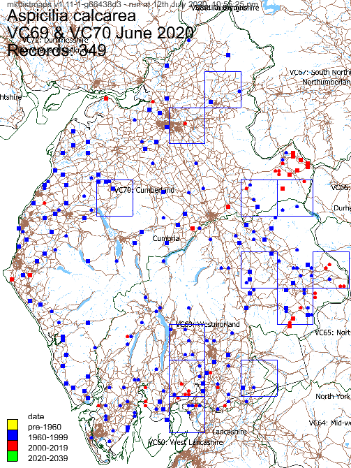
the monad/tetrad is shown as a circle if there is only one record for the monad or tetrad
any records that are only at hectad level are shown as outline squares, rather than filled squares

The mkdistmaps version string and the runtime date and time are added in grey at the top left of each generated map.

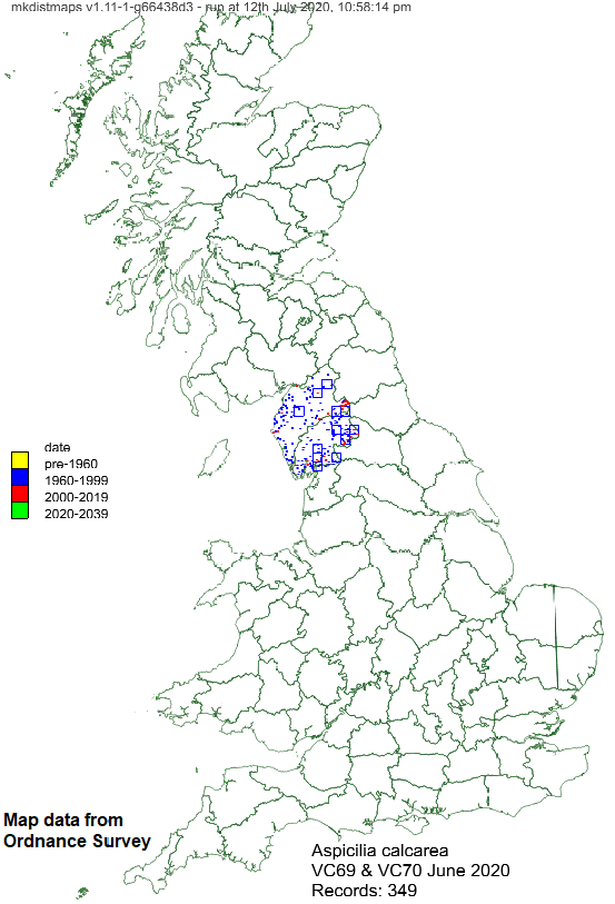
Example monad maps:

Both these monad-level maps use the same data (all records of Aspicilia calcarea in VC69 and VC70, Cumbria, as of June 2020). The first shows the data on a map of Cumbria. The second shows the data on a map of most of Great Britain.

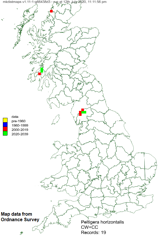
Example hectad map:

This map shows some records of Peltigera horizontalis across GB, displayed at hectad resolution.

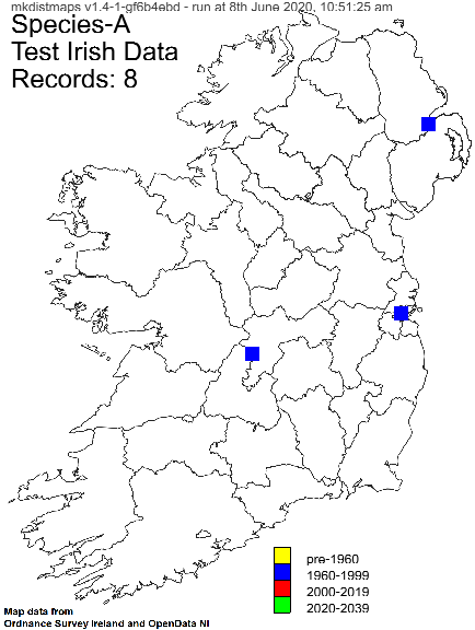
Example Irish hectad map:

Example record and species count maps:

Runtime output

The code generates basic output as it processes the data, finishing like this:

...
Parsed 58248 rows
Errors 1
#0 LC0003050000XIWC Date invalid:undefined Year:NaN
Errors 0
Species: 1,124
Genera: 296
Records: 58,248
Empty rows: 0
Boxes: 998
Runtime: 191 seconds

Usage: GeoJson output

If you set the outputtype to be geojson then geojson format files are generated using standard FeatureCollection, Feature and Polygon object types, with the coordinates output in WGS84 latitude and longitude. Various other objects are also included to help make better maps, ie to give the map a name, show the legend and define popup text for each feature.

A root level style property is defined as per Geojson CSS:

"style": {
  "color": "#000000",
  "fillOpacity": 0.1,
  "weight": 1,
  "opacity": 1
},

In addition, various root properties are set, eg:

"properties": 
{
  "name": "Count of species in each square",
  "set": "VC69 & VC70 June 2020",
  "maptype": "count",
  "datecolours": [],
  "generator": "mkdistmaps v1.13-3-g78cb606 - run at 25th July 2020, 2:58:11 pm",
  "subtitle": "Species: 1,124",
  "countcolours": []
}

Finally, each defined polygon feature may have properties defined, where species is only provided on the "All species" count map.

"properties": {
  "color": "#008000",
  "text": "SD29: 2 species 1944-1946",
  "species": "Arthrorhaphis citrinella|Micarea lignaria var. lignaria"
}

Updates

If the code at github has been updated, you can update your local copy using this command in the mkdistmaps directory:

git pull

You may also need to run this to install any new dependencies:

npm install

Usage: configuration

Specify what you want done in a configuration file. The config file must be in JavaScript Object Notation (JSON) format. The sample config file sample-config.json shows some of the options available.

limit

If you want to test what the maps look like without generating them all, specify the number of species maps that you want to produce, eg 1. Zero means all.

outputFolder

Specify the output folder, which is created if need be

saveSpacesAs

By default, the generated map filenames will contain spaces (if the species names have spaces). If you want these changed, specify an alternative eg _ to use an underscore instead.

recordset

csv - path to csv, optionally including wildcard asterisks
encoding - set CSV file encoding eg to latin1. The default is utf8.
title - text that is added to every generated map
GRCol - name of the CSV column that contains the grid reference
TaxonCol - name of the CSV column that contains the species name
ObsKeyCol - optional name of the CSV column containing an observation key - used to show errors
DateCol - specify either this or YearCol as the name of the CSV column containing the date
YearCol - name of the CSV column containing the year
DateFormats - optional date formats tried. The default is [ "DD/MM/YYYY", "YYYY" ] - see here for format details
headers - optional array of strings containing the CSV column names
renameHeaders - optional specify true to replace the CSV header line with that in headers. The default is false

If your CSV file doesn't contains a header line, then supply the column names in headers.

If your CSV files does contain a header line but it contains duplicate column names, then you can replace it with the column names given in headers and set renameHeaders to true. Here is an example for headers:

[ "Location", "Grid ref", "VC", "checked?", "Recorders", "Date(s)", "Altitude", "Site and visit comments", "BLS no.", "Species", "BLS no.2", "Taxon name", "Group", "Status", "Substrate", "Small scale habitats", "Abundance", "Record notes", "Herbarium", "Specimen", "Determiner" ]

Note: if the CSV file has columns Eastings and Northings then these are cross-checked against the grid reference.

boxSize

Set to hectad, tetrad, monad or all. Default is hectad.

makeGenusMaps

Optionally specify true to make maps for each genus ie the first word of all species names. Default is false.

The genus maps will have "-all" added after the first word (which should result in the genus map displaying first in a directory listing). If there is one record each of "Bacidia" and "Bacidia rubella" then three maps will be produced: "Bacidia", "Bacidia rubella" and "Bacidia -all" with the last one showing 2 records.

makeAllMap

Optionally specify true to make a map for each species found called "All records". Default is false. A map called "All species" is also made if maptype is count

maptype

Optionally specify count to colour squares according to the record-count in each square, using the countcolours ranges. If makeAllMap is true then maps are generated called "All records" and "All species".

The default is date which uses the date or years fields and the datecolours ranges.

outputtype

Optionally specify geojson to make geojson files instead of maps.

geojsonprecision

Optionally specify the precision of coordinates in geojson files. The default of false gives full precision; in practice eg 6 will suffice.

font_filename

Specify the filename of a font eg a TTF file. The tests directory contains an open source font "tests/fonts/SourceSansPro-Regular.ttf".

font_colour

Specify the colour of the written text eg as #000000 or rgba(0,255,0, 1)

basemap

The base map would typically be generated in QGIS using "Export as image", noting the N/W/E/S values

file - path to the base map: must be PNG, JPG or JPEG
north - north bound of supplied base map
west - west bound of supplied base map
east - east bound of supplied base map
south - south bound of supplied base map
scaledown - scale reduction factor for output
showhectadname - set to true to show the hectad name on each map

The following basemap parameters determine where and how descriptive text and the legend are written onto the map

legend_hide - set to true to not show a legend
title_x: X position of start of text. Default: 10
title_y: Y position of start of text. Default: 10
title_y_inc: Y increment for next lines of text. Default: 25
title_fontsize: Title text fontsize. Default: "24pt"
legend_x: X position of start of legend. Default: 10
legend_y: Y position of start of legend. Default: half way down map
legend_inc: Y increment for next legend line. Default: 15
legend_fontsize: Legend text fontsize. Default: "12pt"
hectad_fontsize: Hectad name fontsize. Default: "12pt"

datecolours

Optionally, specify the date range colours. The default is:

[
  { "minyear": 0, "maxyear": 1959, "colour": "rgba(255,255,0, 1)", "legend": "pre-1960" },  // Yellow
  { "minyear": 1960, "maxyear": 1999, "colour": "rgba(0,0,255, 1)", "legend": "1960-1999" }, // Blue
  { "minyear": 2000, "maxyear": 2019, "colour": "rgba(255,0,0, 1)", "legend": "2000-2019" }, // Red
  { "minyear": 2020, "maxyear": 2039, "colour": "rgba(0,255,0, 1)", "legend": "2020-2039" }  // Green
]

countcolours

Optionally, specify the count range colours, using absolute values or percentages. The default is:

[
  { "min": 1, "max": "1%", "colour": "rgba(0,255,0, 1)", "legend': "" },      // Green
  { "min": "1%", "max": "10%", "colour": "rgba(0,0,255, 1)", "legend': "" },  // Blue
  { "min": "10%", "max": "50%", "colour": "rgba(0,0,0, 1)", "legend': "" },   // Black
  { "min": "50%", "max": "100%", "colour": "rgba(255,0,0, 1)", "legend': "" } // Red
]

The legend is built for each map using the actual values, eg "1-1", "2-3", etc. If using percentages, the code ensures that at least one count is in each range, and the legend stops once the maximum is reached.

Used with thanks

A crucial tool is the GeoTools2 code that converts between GB/IE grid references and WGS84 latitude and longitude. I converted this code into a module called geotools2em.js.
Josh Marinacci's pureimage - docs and contributors
C2FO's fast-csv - docs and contributors
Source Sans Pro from Google fonts
Other nodejs modules - see code

I built base maps using QGIS, Ordnance Survey open data, OpenDataNI and Ordnance Survey Ireland open data - thanks.

Vice-county data from https://github.com/BiologicalRecordsCentre/vice-counties and https://github.com/SK53/Irish-Vice-Counties - thanks.

I used data from the British Lichen Society - thanks.

transform tool

transform.js is a command line tool to transform the coordinates within a geojson file from OSGB36 to WGS84

used to convert vice-county boundaries into a format that can be displayed

usage: node transform.js <in.geojson> <out.geojson> <precision>

makerecords tool

makerecords.js is a command line tool which can be used to generate large test CSV data files. The generated records are randomly distributed across the chosen area, ie GB, IE or GB&IE. A linear species distribution is used so very few of some species are likely to be generated, but many more of others. Specify a seed parameter string if you wish to generate a consistent list. The species are given names from the start of an npm word list.

usage: node makerecords.js GB|IE|GBIE <desired-record-count> <species-count> <output-csv-file> <optional-random-seed>

To do

Possibly: write sub-tool to create small geojson files with contours.
Possibly: cope with having Irish and GB grid references displayed on the same map
Possibly: cope with map inserts for out-of-main-area locations
Improve tests, eg split into smaller units
If ReferenceError thrown in test, error not shown but test times out

License

MIT