Features:
- Shot detection
- Logo detection
- Face detection
- Face tracking
- Gender classifier
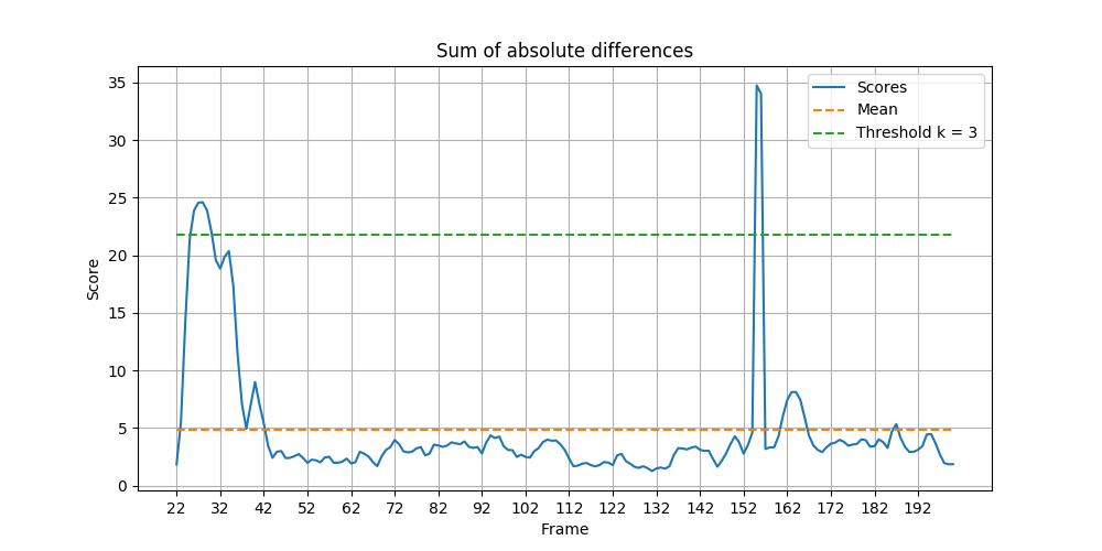
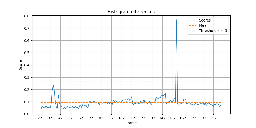
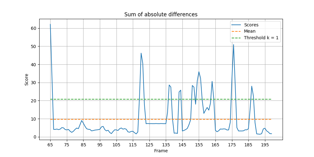
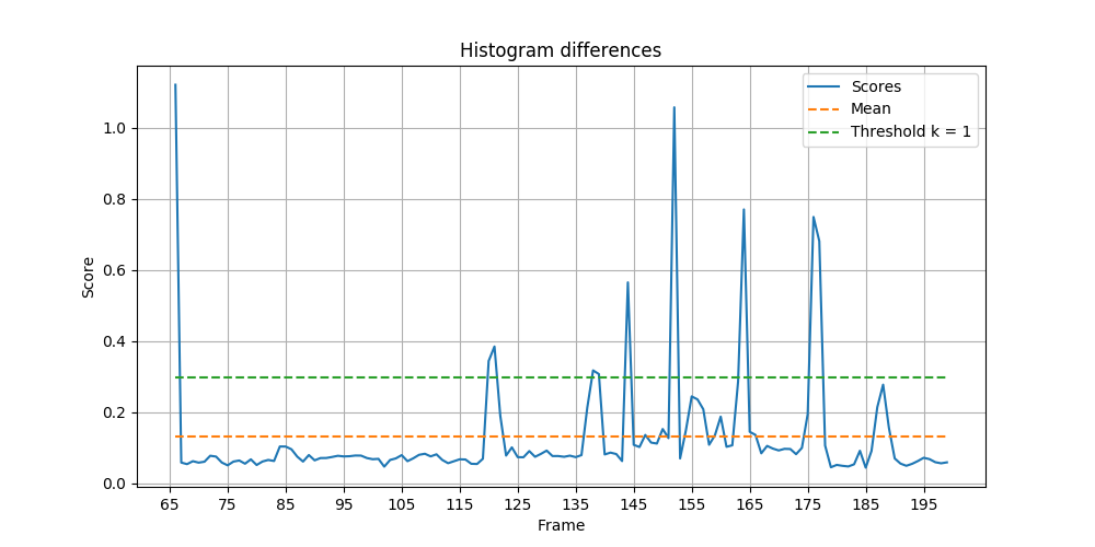
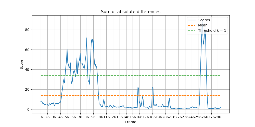
A score is calculated for each frame using either the sum of absolute differences method or the histogram differences method. Given the mean (mu) and standard deviation (sigma) of all the scores, a threshold is chosen as threshold = mu + k x sigma where k is an integer. A shot is a series of frames taken by continuously by one camera. A shot change is declared when the value of the score becomes greater than the threshold and then becomes smaller than the threshold (similar to a peak above the threshold line).
A score is assigned to each frame by calculating the sum of the absolute differences between consecutive frames for every pixel. This value is then normalized by the size of the frame. When the score of a frame is greater than the threshold, a shot change is declared. This method works quite well with simple videos but it is not robust against movements and changes in lighting.
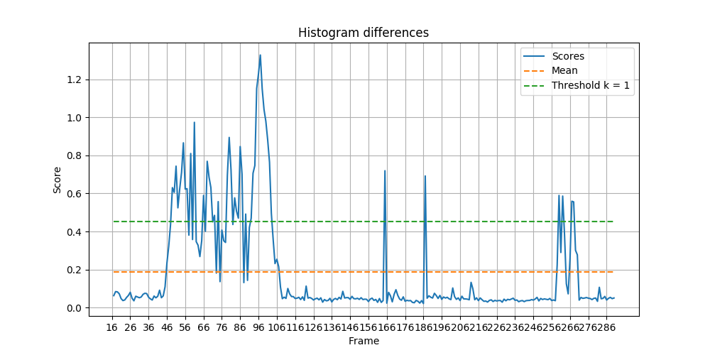
Each frame is converted into a gray-scale image. A histogram with 256 bins, representing all the possible values of a pixel, is created for each frame. Then, a score is assigned by calculating the sum of the absolute differences between histograms of consecutive frames. This method is more robust against small changes in a frame.
Let C be the number of correctly identified cuts,
The two tables below shows the
respective scores for both methods. On average, the histogram
differences (HD) method achieve a higher score across all three metrics
comparing to sum of absolute differences (SAD) method. For example, the
transition from frame 164 (Figure [clip3f164]) to frame 165 (Figure
[fig: clip3f165]) is not detected by the latter but it is by the
former. HD performs especially better in the montage section in clip 3,
where there are frequent shot changes. Also, we see that SAD scored
frame 22 to frame 32 in clip 1 quite high when the man was only moving
to the left of the frame.
| Clip & Correct (C) | Missed (M) | Falsely detected (F) | Recall (V) | Precision (P) | F_1 |
|---|---|---|---|---|---|
| 1 | 1 | 0 | 1 | 1 | 0.5 |
| 2 | 7 | 0 | 2 | 1 | 0.7778 |
| 3 | 5 | 16 | 0 | 0.2381 | 1 |
| Clip & Correct (C) | Missed (M) | Falsely detected (F) | Recall (V) | Precision (P) | F_1 |
|---|---|---|---|---|---|
| 1 | 1 | 0 | 0 | 1 | 1 |
| 2 | 6 | 1 | 1 | 0.8571 | 0.8571 |
| 3 | 15 | 6 | 1 | 0.7142 | 0.9375 |
The relevant code is in shot.py. To get the graphs of shot detection,
run the command below.
python3 run.py shot_detection -t <type> -i <path to frames>To add shot numbers into frames, run the command below. The shot number will appear on the bottom left corner of each frame.
python3 run.py add_shot_numbe -i <input directory> -o <output directory>
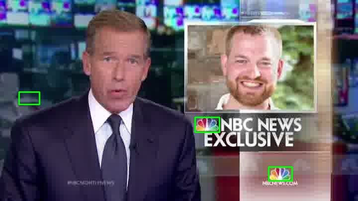
-k <k for thresholding>Template matching is an object detection algorithm which is translation invariant but not scale or rotation invariant. As we are detecting the news company’s logo, we can assume that the target of detection will be in a known orientation. Due to the possibility that there may be multiple occurrences of the logo in a frame, we cannot simply match SIFT features between the logo template and a frame. Template matching is run on templates of different sizes because the size of the logo in a frame is unknown. Then, a score is calculated for all the matches by normalized cross-correlation. The normalized version is chosen because brighter patches will not have a higher score. Also, the score obtained will be in the range [0, 1] and this makes choosing a threshold more intuitive. As the logo in the template and the one in the frame might be slightly different, possibly due to the differences in resolutions or styles, a looser threshold is first used to filter out the irrelevant matches.
For each match, if its score is greater than the loose threshold, it is kept. Then, the algorithm checks if that particular match is a slight translation of a match we have already decided to keep. If it is, the match is discarded. This prevents having multiple boxes around one logo. Afterwards, SIFT descriptors are calculated for the remaining matches and a score is calculated using feature matching and Lowe’s ratio test with the logo template. If a match’s score is above a different threshold, it is declared as a match of the template and a box is put around the match.
Initially, I only did one pass with either normalized cross-correlation
or SIFT feature matching. However, this led to fairly poor results, with
the algorithm often unable to detect multiple logos and including many
irrelevant matches. Therefore, the two passes approach, first with a
looser threshold using normalized cross-correlation and then with
another threshold with SIFT feature matching, is used. SIFT is scale and
rotation invariant. Therefore, it will not penalize logos that have
slight size differences to the template. This is good because even if we
have multiple scales, they might not be an exact match in size. As can
be seen in Figure [fig: logogood], the algorithm can detect multiple
logos. In hindsight, it would have been more efficient to scale down the
images to multiple scales instead of scaling down the templates. This is
because sliding the template across the image takes much longer than
resizing every frame to different scales.
The relevant code is in logo.py. To run logo detection, run the
command below.
python3 run.py logo_detection -i <input directory> -o <output directory>
-d <logo path> -t <min threshold for NCC>There are 260 images in the female and male classes respectively. Each
image is accompanied by a .mat file specifying the coordinates of the
left eye, right eye, nose and mouth. The following rules are used to
crop the images in order to obtain the faces.
The relevant code for face cropping is in crop_images() in face.py.
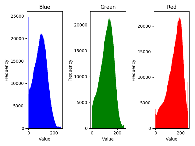
The initial attempt to detect faces is to use skin detection - trying to
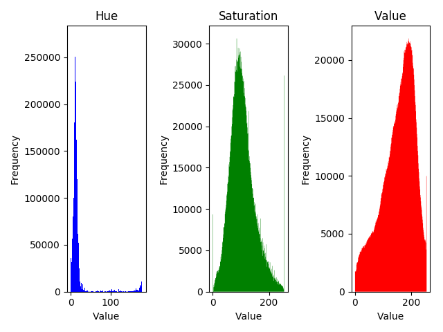
filter out skin in images. Figure [fig: rgb] and Figure [fig: hsv] show
the color distributions of faces in RGB and HSV color spaces. The HSV
color space has narrower distributions, especially with hue. Although
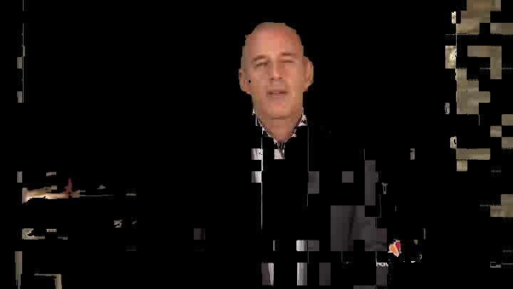
this method works sometimes as seen in Figure [fig: hsvgood], it is
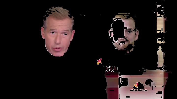
not successful in general. It fails to detect a large area of the face
of the man on the right in Figure [fig: hsvbad] and includs a lot of
the background.This model is especially poor when other things in the
frame are very similar to human skin tone.
The relevant code for HSV face detection is in
visualize_distributions() and face_detection_hsv() in face.py.
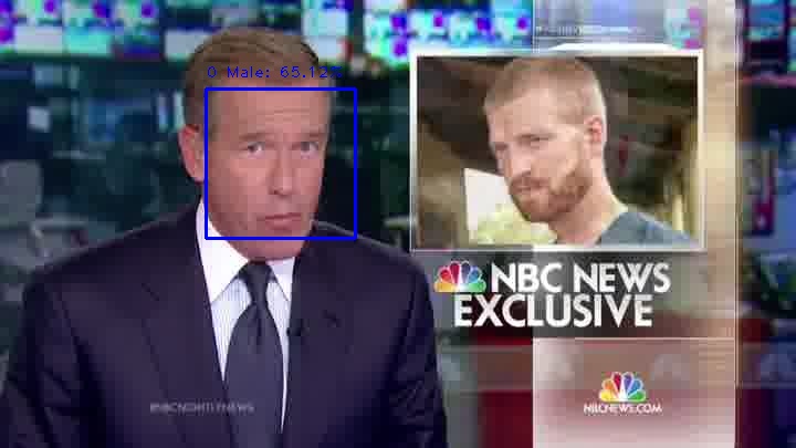
I ended up using cv2.CascadeClassifier for detecting faces. The full
name of this classifier is Haar feature-based cascade classifier for
object detection. It is a OpenCV pre-trained classifier for face stored
in an XML file. It works fairly well. It has no trouble detecting
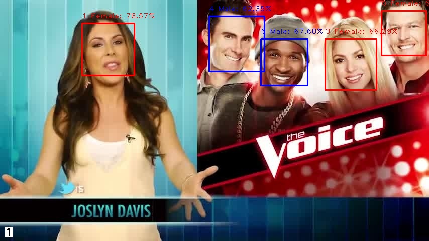
multiple people in a frame or people of colour, like in Figure [fig:
facegood]. However, it is usually unable to detect faces turned to the
side. The detector was unable to detect the person on the left in any of
the frames he appeared in that particular position in Figure [fig:
facebad].
After obtaining the faces in a frame, for each face in the current frame, the SIFT descriptors are found. Then, they are matched to the SIFT descriptors of all the faces in the previous frame using feature matching and Lowe’s ratio test. Then, a score is obtained from the number of matches. If the score is above a set threshold, the algorithm declares that the face we are looking at is found in the previous frame and we will display the index assigned to that particular face in the previous frame. If the face is not found, we assign a new index to the face. The index of each face is labelled on top of the box.
90% of the images (234 images from each class) are used for training, whereas the other 10% (26 images from each class) are used for testing the accuracy of the model. The accuracy is defined as the percent of correctly identified faces, not SIFT descriptors, in the cases of support-vector machine and neural network.
The SIFT descriptors of the training images are passed into the SVM model for training. A radial basis function kernel is used. Then, for each detected face in a frame, the SIFT descriptors are extracted and fed to the trained SVM model. A prediction for each descriptor is obtained. If more descriptors are predicted as female than male, the image is classified as female. If more descriptors are predicted as male than female, the image is classified as male. If there are equal number of descriptors being predicted as both female and male, the image is then classified as unknown.
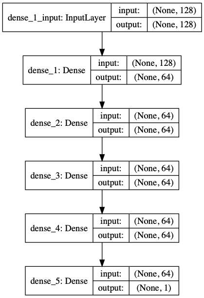
The same as SVM, except with a neural network model instead. The model
uses a binary crossentropy loss, adam for optimization, and accuracy as
the metric. The neural network used is shown in Figure [fig: nnmodel].
All the training and testing images are padded with black borders to
obtain a square shape and then resized to be 72 pixels by 72 pixels. The
training images are then passed to the CNN model shown in Figure [fig:
cnnmodel] for training. The model uses a binary crossentropy loss,
stochastic gradient descent for optimization, and accuracy as the
metric. Each detected face is padded to obtain a square shape. Then, the
image is resized to be 72 pixels by 72 pixels. The resized image is then
passed to the trained CNN model and a category prediction is obtained.
The relevant code for training any of the three models is in
train_model() in face.py. To train a gender classification model,
run the command below.
python3 run.py train -m <model path after training>
-c <classification model (SVM, NN_SIFT, or CNN)>
The relevant code for face detection (including gender classification
and face tracking) is in face_detection() in face.py. Run the
command below.
python3 run.py face_detection -i <input directory> -o <output directory>
-c <classification model (SVM, NN_SIFT, or CNN)> -m <trained model path>
-s <min size for face detection> The table below shows the test accuracies of the three models. As expected, CNN performed poorly, achieving an accuracy that is equivalent to random guesses, due to the very small training data size of 468. It consistently classify all the faces as either female and male.
| Model | Description | Accuracy on test set |
|---|---|---|
| SVM | Using SIFT descriptors of faces | 100.00% |
| Neural network | Using SIFT descriptors of faces | 92.30% |
| CNN | Using cropped and resized faces | 50.00% |
The relevant code for combining all the frames to a video is in
make_video() in utils.py. To do logo detection, face detection, face
tracking and gender classification and make a video, run the command
below.
python3 run.py run_all -i <input directory> -o <output directory>
-d <logo path> -t <min threshold for NCC> -m <trained model path>
-c <classification model (SVM, NN_SIFT, or CNN)> -v <name of output video>
-f <frame per second> -s <min size for face detection>Video shot boundary detection based on color histogram
