This is an example project showing the usage of the CMSIS-Stream software component.
It is the original uVision DSP_App demo converted to CMSIS-DSP Compute Graph.
The implemented graph is:
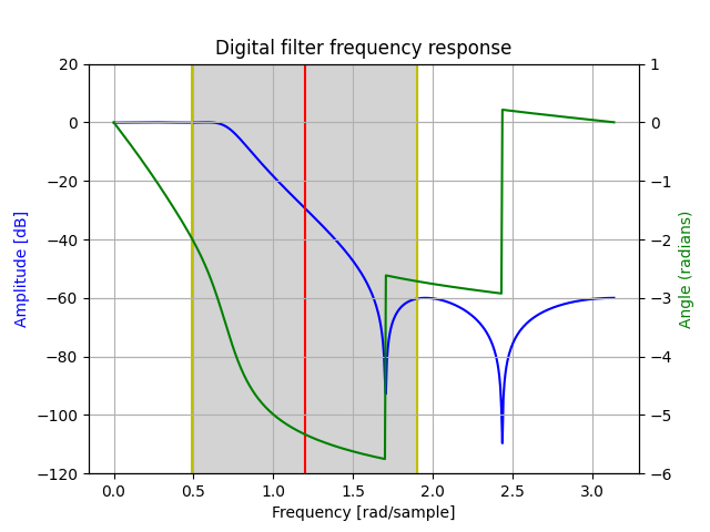
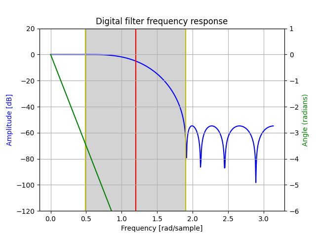
The filter will show an attenuation for some frequencies and not others.
EOUT is the amplitude of the filtered signal (root mean square with DC offset removed).
TOUT is the comparison with a threshold to detect the presence of a specific frequency band in the signal.
The nodes in the graph are:
adc: Get the input signal data from the timer interrupttoFixedPoint: Convert samples toq15_tiir: The IIR filter (can be replaced by the FIR by changinggraph.py)toFloat: convert sample tofloat32_tdac: Generate the output signal for use in the timer interruptrms: Compute the root mean square on a window of sample. The DC offset is removed before the computationthreshold: Compare the value with a threshold. Return0x7FFFwhen input value>=to the threshold. Otherwise return0.amplitude_log: Write to a global variable monitored by the logic analyzerthreshold_log: Write to a global variable monitored by the logic analyzer
When the application is running in uVision, you should see:
The generated signal can be changed by using a toolbox window displayed in uVision:
The event recorder window displays Compute graph events and timer events:
- Start of a new schedule iteration
- Execution of a compute graph node
- AD conversion in timer interrupt
- DA conversion in timer interrupt
This trace can be used to track real-time issues.
The IIR (or FIR) nodes are just wrappers around the implementation of the original demo files : DSP_FIR.c and DSP_IIR.c
As consequence, those wrappers have no argument to specify the filter coefficients since they are hard coded in the original filters.
A future version may use a more customizable wrapper.
The DAC / ADC data is coming from the TIMER2_IRQHandler in DSP_App.c
The original application was containing several cases (controlled with #if) to select a format f32, q31,q15. But the original sample was always f32.
This version is extracting the conversion that is now part of the graph and made explicit. There is no more the need of compilation flags to select the data format. But the graph needs to be regenerated with another data format using the python script graph.py
Same to switch between IIR or FIR : the graph needs to be regenerated.
The original version is using 256 samples for all the blocks. To demonstrate the flexibility introduced with the compute graph, there is a different graph where all blocks (except sink / source) are using 192 samples. (graph described with the script graph_with_higher_latency.py)
It introduces an additional latency in the system since sometime the scheduling is requiring 2 calls to the source or 2 calls to the sink.
This is handled thanks to the ADC / DAC nodes that are connected to the interrupt handler through queues. The depth of the queue is controlled by AUDIO_QUEUE_DEPTH in the file globalCGSettings.h. This value must be coherent with the generated scheduling to avoid overflow or underflow in the sources / sinks.
This latency can be analyzed by using a compute graph doing nothing (adc connected directly to the dac) and using the square signal generator in the toolbox.
In the previous picture, one can see that the output signal is delayed from the input by 3 DSP packets.
The AUDIO_QUEUE_DEPTH is 3 for this example.
AUDIO_QUEUE_DEPTH must always be >= 2 because when the system starts you must be able to generate a packet although you have not received the first one needed to start the computation. A first dummy packet is used.
Then, as soon as you have received the first DSP packet, the computation is starting but at same time the system is also starting to generate the second output packet.
So, the first useful packet resulting from the computation is the 3rd packet generated on the output : a delay of 2 packets compared to the input.
In case where the scheduling in calling the source or sink several time in sequence, you have additional latencies like in the example above where the total latency is not 2 but 3.
In below plots, the gray area represents the frequencies covered by the sweep sine and the red vertical line representes the middle of this area.
python iir_filter_design.py -p
python fir_filter_design.py -p
python iir_filter_design.py creates DSP_IIR.c
python fir_filter_design.py creates DSP_FIR.c
From the ComputeGraph folder do:
python graph.py to generate the simpler DSP graph with minimum latency
python graph_with_higher_latency.py to generate a graph with higher latency
python graph_latency_study.py to generate a graph to study the latency
Above commands are generating ComputeGraph/dsp_scheduler.cpp and also a graphviz file for graphical representation:
ComputeGraph/Pictures/graph.dotComputeGraph/Pictures/graph_with_higher_latency.dotComputeGraph/Pictures/graph_latency_study.dot
A dot file can be converted to a png using the graphviz command dot:
dot -Tpng -o Pictures\graph.png Pictures\graph.dot
The python scripts can take some options:
python graph.py --fir to use a FIR instead of IIR
python graph.py --f32 to use float instead of q15_t for the processing.


