Time series analysis today is an important cornerstone of quantitative science in many disciplines, including natural and life sciences as well as economics and social sciences. Regarding diverse phenomena like tumor cell migration, brain activity and stock trading, a similarity of these complex systems becomes apparent: the observable data we measure – cell migration paths, neuron spike rates and stock prices – are the result of a multitude of underlying processes that act over a broad range of spatial and temporal scales. It is thus to expect that the statistical properties of these systems are not constant, but themselves show stochastic or deterministic dynamics of their own. Time series models used to understand the dynamics of complex systems therefore have to account for temporal changes of the models' parameters.
bayesloop is a python module that focuses on fitting time series models with time-varying parameters and model selection based on Bayesian inference. Instead of relying on MCMC methods, bayesloop uses a grid-based approach to evaluate probability distributions, allowing for an efficient approximation of the marginal likelihood (evidence). The marginal likelihood represents a powerful tool to objectively compare different models and/or optimize the hyper-parameters of hierarchical models. To avoid the curse of dimensionality when analyzing time series models with time-varying parameters, bayesloop employs a sequential inference algorithm that is based on the forward-backward-algorithm used in Hidden Markov models. Here, the relevant parameter spaces are kept low-dimensional by processing time series data step by step. The module covers a large class of time series models and is easily extensible.
bayesloop has been successfully employed in cancer research (studying the migration paths of invasive tumor cells), financial risk assessment, climate research and accident analysis. For a detailed description of these applications, see the following articles:
Bayesian model selection for complex dynamic systems
Mark C., Metzner C., Lautscham L., Strissel P.L., Strick R. and Fabry B.
Nature Communications 9:1803 (2018)
Superstatistical analysis and modelling of heterogeneous random walks
Metzner C., Mark C., Steinwachs J., Lautscham L., Stadler F. and Fabry B.
Nature Communications 6:7516 (2015)
- infer time-varying parameters from time series data
- compare hypotheses about parameter dynamics (model evidence)
- create custom models based on SymPy and SciPy
- straight-forward handling of missing data points
- predict future parameter values
- detect change-points and structural breaks in time series data
- employ model selection to online data streams
For a comprehensive introduction and overview of the main features that bayesloop provides, see the documentation.
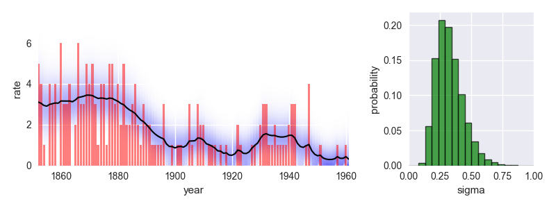
The following code provides a minimal example of an analysis carried out using bayesloop. The data here consists of the number of coal mining disasters in the UK per year from 1851 to 1962 (see this article for further information).
import bayesloop as bl
import matplotlib.pyplot as plt
import seaborn as sns

S = bl.HyperStudy()  # start new data study
S.loadExampleData()  # load data array

# observed number of disasters is modeled by Poisson distribution
L = bl.om.Poisson('rate')

# disaster rate itself may change gradually over time
T = bl.tm.GaussianRandomWalk('sigma', bl.cint(0, 1.0, 20), target='rate')

S.set(L, T)
S.fit()  # inference

# plot data together with inferred parameter evolution
plt.figure(figsize=(8, 3))

plt.subplot2grid((1, 3), (0, 0), colspan=2)
plt.xlim([1852, 1961])
plt.bar(S.rawTimestamps, S.rawData, align='center', facecolor='r', alpha=.5)
S.plot('rate')
plt.xlabel('year')

# plot hyper-parameter distribution
plt.subplot2grid((1, 3), (0, 2))
plt.xlim([0, 1])
S.plot('sigma', facecolor='g', alpha=0.7, lw=1, edgecolor='k')
plt.tight_layout()
plt.show()
This analysis indicates a significant improvement of safety conditions between 1880 and 1900. Check out the documentation for further insights!
The easiest way to install the latest release version of bayesloop is via pip:
pip install bayesloop
Alternatively, a zipped version can be downloaded here. The module is installed by calling python setup.py install.
The latest development version of bayesloop can be installed from the master branch using pip (requires git):
pip install git+https://github.com/christophmark/bayesloop
Alternatively, use this zipped version or clone the repository.
bayesloop is tested on Python 3.8. It depends on NumPy, SciPy, SymPy, matplotlib, tqdm and cloudpickle. All except the last two are already included in the Anaconda distribution of Python. Windows users may also take advantage of pre-compiled binaries for all dependencies, which can be found at Christoph Gohlke's page.
bayesloop supports multiprocessing for computationally expensive analyses, based on the pathos module. The latest version can be obtained directly from GitHub using pip (requires git):
pip install git+https://github.com/uqfoundation/pathos
Note: Windows users need to install a C compiler before installing pathos. One possible solution for 64bit systems is to install Microsoft Visual C++ 2008 SP1 Redistributable Package (x64) and Microsoft Visual C++ Compiler for Python 2.7.
If you have any further questions, suggestions or comments, do not hesitate to contact me: bayesloop@gmail.com


