
In this repository, you can find my works related to a bunch of different self paced machine learning projects. Since I have passion for ML and Data Mining, I got my hands dirty to get hands-on experiences.
Please, check out once the table to get briefly information about projects, below.
| Problem | Methods | Libs | Repo |
|---|---|---|---|
Prediction Skip Action on Music Dataset |
LightGBM, Linear Reg, Logistic Reg. |
Sklearn, LightGBM, Pandas, Seaborn |
Click |
| Hairstyle Classification | LightGBM, TF-IDF |
Sklearn, LightGBM, Pandas, Seaborn |
Click |
| Time Series Analysis by SARIMAX | ARIMA, SARIMAX |
statsmodels, pandas, sklearn, seaborn |
Click |
| Multi-language and Multi-label Classification Problem on Fashion Dataset | LightGBM, TF-IDF |
Sklearn, LightGBM, Pandas, Seaborn |
Click |
| Which one does it catch whole* SPAM SMS? | Naive Bayesian, SVM, Random Forest Classifier, Deep Learning - LSTM, Word2Vec |
Sklearn, Keras, Gensim, Pandas, Seaborn |
Click |
| Which novel do I belong To? | Deep Learning - LSTM, Word2Vec |
Sklearn, Keras, Gensim, Pandas, Seaborn |
Click |
| Why do customers choose and book specific vehicles? | Random Forest Classifier |
Sklearn, Pandas, Seaborn |
Click |
| Forecasting impact of promos (promo1, promo2) on sales in Germany, Austria, and France | Random Forest Regressor, ARIMA, SARIMAX |
statsmodels, pandas, sklearn, seaborn |
Click |
| Random Forest Classification Tutorial in PySpark | Random Forest Classifier |
Spark (PySpark), Sklearn, Pandas, Seaborn |
Click |
| Spatial data enrichment: Join two geolocation datasets by using Kdtree | Kd-tree |
cKDTree |
Click |
| Implementation of K-Means Algorithm from scratch in Java | K-Means |
Java SDK |
Click |
| Forecasting AWS Spot Price by using Adaboosting on Rapidminer | Adaboost Classifier, Decision Tree |
Rapidminer |
Click |
Please, scroll down to see the comprehensive details about projects or visit their repository.
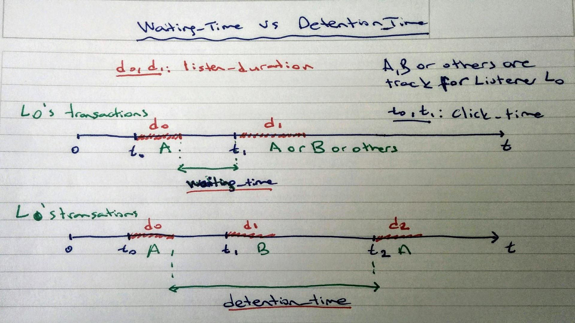
Since we don't have any class already labelled and any continuous target variable, we need to pick a feature for our target feature to predict skipping action of listener. According to the features we created, per_listen will be more suitable for that problem since it obviously gives idea about skipping action. If we pick it as a target feature, this problem will turn out a scoring/probability problem because of having ratio of listening time, which tends between 0 to 1.
If we want to convert that problem to a classfication problem, we can determine a treshold for skipping aciton as a rule of thump. per_listen denotes how much percentage of the track that were listened by listener. So, our threshold could be 25%, 50% even 51% and so on. However, before making a decision, we can check out Complementary Cumulative Distribution Function (CCDF) of per_listen. It would be give an idea about our reasonanle threshold. According the following plot, we have 65% of instances, whose per_listen value is greater than 0.5. Therefore, 0.5 is reasonable, however, when we think about it more realistic, less than 0.5 around 0.25 would be more suitable determine any skipping action.

The dataset contains a sample 10000 images mined from Instagram and clustered based on the hairstyle they showcase.
The variable cluster represents the hairstyle cluster that the image has been assigned to by
the visual recognition algorithm.
Each row contains the variable url which is the link to the image and the number of likes
together with the comments per image. The user_id is the unique id of the Instagram account
from which the post comes and the variable id is the unique identifier associated with the post
itself.
Each post contains the date(date_unix) in unix format when the image was posted on
Instagram and additionally the date has been converted to different formats (date_week->non-iso number of the week, date_month -> the month, date_formated ->full date dd/mm/YY) partly
for use in prior analyses. Feel free to convert that variable in a way that suits your analysis.
Additionally a classifier influencer_flag was added to each of the images which have more than
500 likes, flagging them as influencer posts.

In this experiment, we use time series analysis technique to decompose our data into 3 components like the below:
1-Trend (T)
2-Seasonility (S)
3-Residual (R)
Once we need to get a statinory dataset before performing Time Series Analysis (TSA) flawlessly beacuse it would be easy making a predicition over a stationary dataset since it would already satisfy the preoperties of Normal Distribution in terms of mean and variance, roughly. So, we need to delve into the raw dataset by applying some EDA techniques to expose valuable insight of data related to trend, and seasonility if it is possible to observe in EDA. After we complete data analyis stage, we need to pick best available techniques (e.g ARIMA, SARIMAX) to perform on the dataset according to our knowledge we would get in EDA.
In EDA stage, we will be applying a bunch of techniques such as, boxploting, rolling statictics (mean, std) by time based features (year, month, day, weekday and quarter) to find out 2 components (trend, seasonility) out of 3 time series components over specific plots, rougly. Those plots will give reasonable feedback for TSA before starting it.
In TSA stage, we will build different models for non-seasonal and seasonal approahes by using ARIMA and SARIMAX in statsmodels package, respectively.
Since the most challenging parts of TSA is finding optimum parameters (p,d,q) and (P,D,Q,S) of those techniques, we will be referring to Autocorrelation (ACF) and Partial Autocorrelation (PACF) functions to find out significant time correlations in terms of performing either Autoregression Model (AR) or Moving Average Model (MA), or Seanosal Autoregression (SAR) and Moving Average (SAM).

Dataset was collected over different fashion web sites. It consists of 7 fields like below.
id: A unique product identifiername: The title of the product, as displayed on our websitedescription: The description of the productprice: The price of the productshop: The shop from which you can buy this productbrand: The product brandlabels: The category labels that apply to this product
The text features (name, description) are in different languages, such as English, German and Russian. The format of target feature is multilabels (60 categories) that were tagged according to corresponding to the category in fashion web sites differently.

| Problem | Data | Methods | Libs | Link |
|---|---|---|---|---|
NLP |
Text | Naive Bayesian, SVM, Random Forest Classifier, Deep Learning - LSTM, Word2Vec |
Sklearn, Keras, Gensim, Pandas, Seaborn |
https://github.com/erdiolmezogullari/ml-spam-sms-classification |
In this project, We applied supervised learning (classification) algorithms and deep learning (LSTM).
We used a public SMS Spam dataset, which is not purely clean dataset. The data consists of two different columns (features), such as context, and class. The column context is referring to SMS. The column class may take a value that can be either spam or ham corresponding to related SMS context.
Before applying any supervised learning methods, we applied a bunch of data cleansing operations to get rid of messy and dirty data since it has some broken and messy context.
After obtaining cleaned dataset, we created tokens and lemmas of SMS corpus seperately by using Spacy, and then, we generated bag-of-word and TF-IDF of SMS corpus, respectively. In addition to these data transformations, we also performed SVD, SVC, PCA to reduce dimension of dataset.
To manage data transformation in training and testing phase effectively and avoid data leakage, we used Sklearn's Pipeline class. So, we added each data transformation step (e.g. bag-of-word, TF-IDF, SVC) and classifier (e.g. Naive Bayesian, SVM, Random Forest Classifier) into an instance of class Pipeline.
After applying those supervised learning methods, we also perfomed deep learning. Our deep learning architecture we used is based on LSTM. To perform LSTM approching in Keras (Tensorflow), we needed to create an embedding matrix of our corpus. So, we used Gensim's Word2Vec approach to obtain embedding matrix, rather than TF-IDF.
At the end of each processing by different classifier, we plotted confusion matrix to compare which one the best classifier for filtering SPAM SMS.

| Problem | Data | Methods | Libs | Link |
|---|---|---|---|---|
NLP |
Text | Deep Learning - LSTM, Word2Vec |
Sklearn, Keras, Gensim, Pandas, Seaborn |
https://github.com/erdiolmezogullari/ml-deep-learning-keras-novel |
This project is related to text classification problem that we tackled with Deeplearing (LSTM) model, which classifies given arbitrary paragraphes collected over 12 different novels randomly, above:
1. alice_in_wonderland
2. dracula
3. dubliners
4. great_expectations
5. hard_times
6. huckleberry_finn
7. les_miserable
8. moby_dick
9. oliver_twist
10. peter_pan
11. talw_of_two_cities
12. tom_sawyer
In other words, you can think about those novels are our target classes of our dataset.
To distinguish actual class of paragraph, the semantic latent amongst paragraphes would play an important role. Therefore, We used Deeplearing (LSTM) on top of Keras (Tensorflow) after creating an embedding matrix by Gensim's word2vec.
If there is any semantic latent amongst sentences in corresponding paragraph, We think about similar paragraphes were collected from same resources (novels) most likely.

| Problem | Data | Methods | Libs | Link |
|---|---|---|---|---|
Imbalanced Data |
Car Booking | Random Forest Classifier |
Sklearn, Pandas, Seaborn |
https://github.com/erdiolmezogullari/ml-imbalanced-car-booking-data |
We built a machine learning model that answers the question, -what is the customer preference- on car booking dataset.
We explored the dataset by using Seaborn, and transformed, derived new features necessary.
In addition, the shape of dataset is imbalanced. It means that the target variable's distribution is skewed. To overcome that challenge, there are already defined a few different techniques (e.g. over/under re-sampling techniques) and intuitive approaches. We try to solve that problem using resampling techniques, as well.

| Problem | Data | Methods | Libs | Link |
|---|---|---|---|---|
Forecasting - Timeseries |
Sales | Random Forest Regressor |
statsmodels, pandas, sklearn, seaborn |
https://github.com/erdiolmezogullari/ml-time-series-analysis-on-sales-data |
There are stores are giving two type of promos such as radio, TV corresponding to promo1 and promo2 so that they want to increase their sales across Germany, Austria, and France. However, they don't have any idea about which promo is sufficient to do it. So, the impact of promos on their sales are important roles on their preference.
To define well-defined promo strategy, we once need to analysis data in terms of impacts of promos. In that case, since data is based on time series, we once referred to use time series decomposition. After we decomposed observed data into trend, seasonal, and residual components, We exposed the impact of promos clearly to make a decision which promo is better in each country.
In addition, we used Random Forest Regression in this forecasting problem to boost our decision.

| Problem | Data | Methods | Libs | Link |
|---|---|---|---|---|
ML Service |
Randomly Generated | Random Forest Classifier |
Flask, Docker, Redis, Sklearn |
https://github.com/erdiolmezogullari/ml-dockerized-microservice |
In this project, a ML based micro-service was developed on top of REST and Docker after building a machine learning model by performing Random Forest
We used docker-compose to launch the micro services, below.
1.Jupyter Notebook,
2.Restful Comm. (Flask),
3.Redis
After we created three different container, our MLasS would be ready.

| Problem | Data | Methods | Libs | Link |
|---|---|---|---|---|
PySpark |
Randomly Generated | Random Forest Classifier |
Spark (PySpark), Sklearn, Pandas, Seaborn |
https://github.com/erdiolmezogullari/ml-random-forest-pyspark |
In this repository, you can find a bunch of sample code related to how you can use PySpark Spark's MLlib (Random Forest Classifier), and Pipeline via PySpark.

| Problem | Data | Methods | Libs | Link |
|---|---|---|---|---|
Data Enrichment |
Spatial | Kd-tree |
cKDTree |
https://github.com/erdiolmezogullari/ml-join-spatial-data |
In this project, to build an efficient script that finds the closest airport to a given user based on their geolocation and the geolocation of the airport.
To make that data enrichment, we used Kd-tree algorithm.

| Problem | Data | Methods | Libs | Link |
|---|---|---|---|---|
Implementation |
Statistics of Countries | K-Means |
Java SDK |
https://github.com/erdiolmezogullari/ml-k-means |
Dataset: https://en.wikibooks.org/wiki/Data_Mining_Algorithms_In_R/Clustering/K-Means#Input_data
| Problem | Data | Methods | Libs | Link |
|---|---|---|---|---|
Forecasting, Timeseries Analysis |
AWS EC2 Spot Price | Adaboost Classifier, Decision Tree |
Rapidminer |
https://github.com/erdiolmezogullari/ml-forecasting-aws-spot-price |
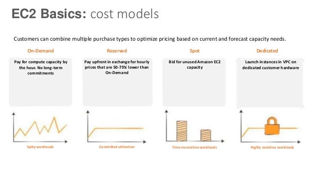
In our project, we will use public data, which was collected by third party people and released through some specific websites. Since our data will be mainly related to Amazon Web Services’ (AWS) Elastic Computing (EC2), it will be consisting of some different fields. EC2 is a kind of virtual machine in the AWS’s cloud. A virtual machine can be created just in time either on private or public cloud over AWS whenever you need it. A new virtual machine can be picked with respect to different specs and configurations in terms of CPU, RAM, storage, and network band limit before creating it once from scratch. EC2 machines also are separated and managed by AWS on different geographical regions (US East, US West, EU, Asia Pacific, South America) and zone to increase availability of virtual machines across the world. AWS has different segmentations, which were classified with respect to system specs by AWS for based on different goals (macro instance, general purpose, compute optimized, storage optimized, GPU instance, memory optimized). Payment options are dedicated, ondemand and spot instance. Since they make different cost to customer’s operation, customers may prefer different kinds of virtual machine according to their goals and budgets. In general, spot instance is cheaper than the rest of the options. However, spot instance may be interrupted if market price exceeds our max bid. In our research, we will focus on spot instance payment. Our aim in this project will be selecting correct AWS instance from the Spot Instance Market according to the requirement of the customer. We plan to perform Decision Tree on streaming data to make a decision on the fly. It may be implemented as an incremental version of decision tree since data is changing continuously