sf2turbo

Intro

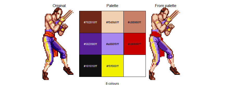
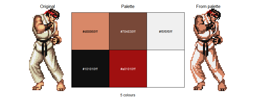
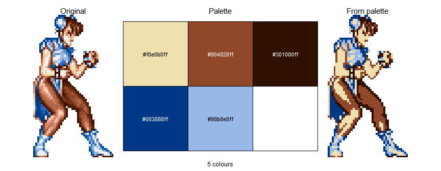
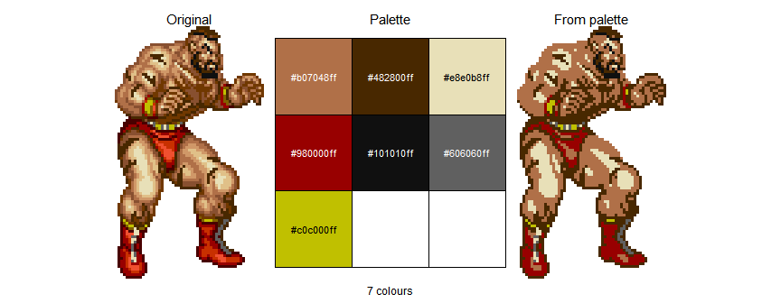
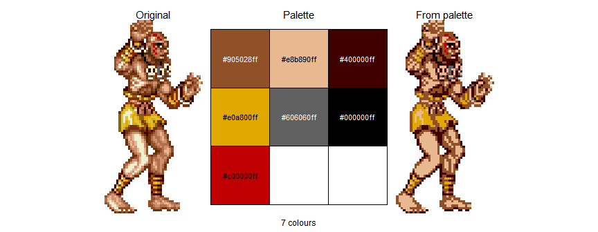
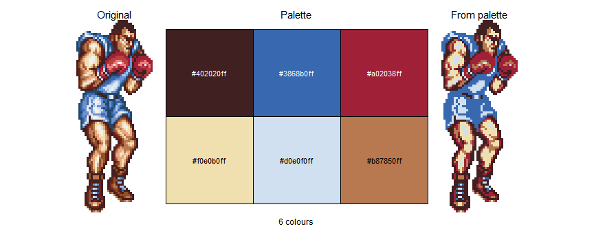
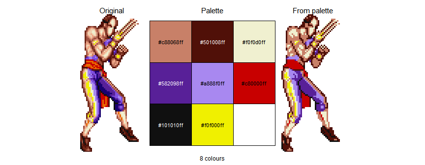
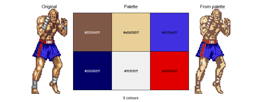
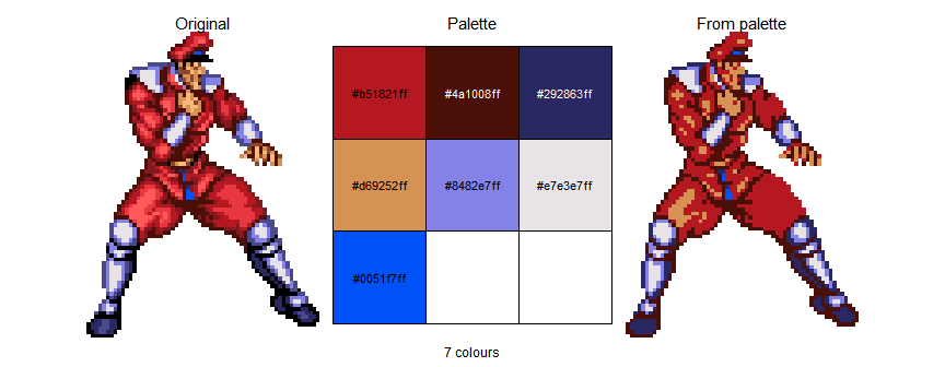
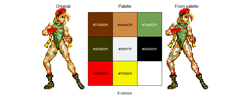
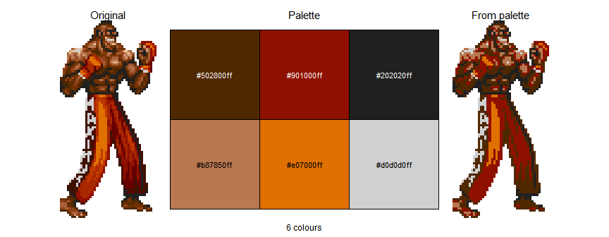
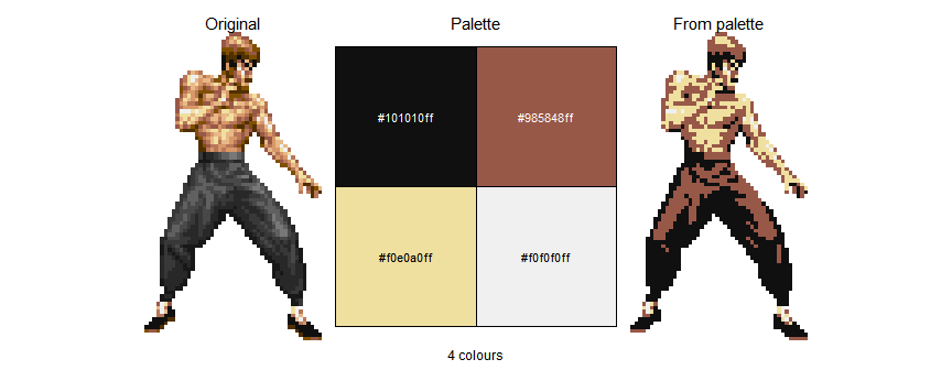
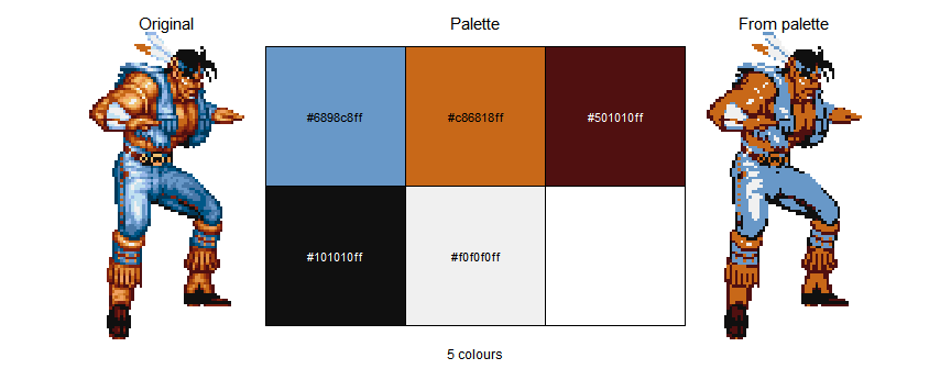
This is an exploratory look at extracting colours from Super Street Fighter 2 character sprites in order to make colour palettes.
It’s just for fun and has some pretty serious flaws (and is also very inefficient)
Executive summary: colours are hard

library(tidyverse)
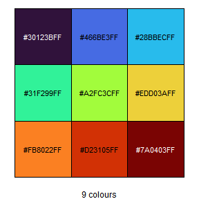
library(magick)

Approach

Function to visualise colours

Start by writing a function that allows me to visualise a vector of colours
This is for convenience and will be super useful later on

view_palette <- function(cols, lab_size = 3){
  
  n <- length(cols)
  nc <- ceiling(sqrt(n))
  nr <- ceiling(n/nc)
  n_extra <- (nc*nr) - n
  v <- col2rgb(cols) %>% rgb2hsv() %>% magrittr::extract(3,)  
  
  tidyr::crossing(x=1:nc, y=1:nr) %>% 
    dplyr::arrange(desc(y), x) %>% 
    dplyr::mutate(pal = c(cols, rep("transparent", n_extra)),
                  v = c(v, rep(NA, n_extra)),
                  lab_col = dplyr::case_when(is.na(v) ~ "transparent",
                                             v > 0.7 ~ "Black",
                                             TRUE ~ "White")) %>% 
    ggplot2::ggplot()+
    ggplot2::geom_tile(ggplot2::aes(x,y,fill=I(pal)), col=1)+
    ggplot2::geom_text(ggplot2::aes(x,y,label=pal, col=I(lab_col)), size = lab_size)+
    ggplot2::coord_equal()+
    ggplot2::theme_void()+
    ggplot2::theme(plot.caption = ggplot2::element_text(hjust = 0.5))+
    ggplot2::labs(caption = paste0(n, " colours"))
}

# Test output
view_palette(viridis::turbo(9))

Read image

Read a test image to develop some working code with

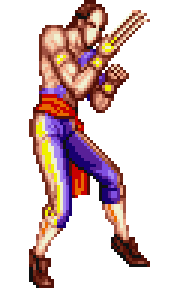
i <- image_read('files/vega.png')
image_ggplot(i)

Extract colours

Convert the image to a tidy, long format raster dataframe (removing transparent pixels)
Append the LAB colour model values in their own columns

# Convert to raster and compute LAB values
ir <-
  i %>% 
  image_raster() %>%
  as_tibble() %>% 
  filter(col != "transparent") %>% 
  transmute(col2rgb(col) %>% 
              t() %>% 
              farver::convert_colour(from = "rgb", to = "lab") %>% 
              as_tibble())

Compute the distance of each colour to every other colour
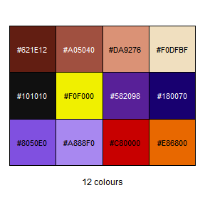
Use hierarchical clustering to extract 12 colours (I think these sprites only contain 15 colours anyway!)

clusts <- dist(ir, method = "maximum") %>% hclust(method = "complete")

# Compute colours from clusters
cols_df <-
  ir %>%
  mutate(group = cutree(clusts, k=12)) %>%
  group_by(group) %>%
  summarise(across(c(l,a,b), mean), .groups = "drop") %>%
  select(-group)

# All colours
all_cols <- cols_df %>% farver::encode_colour(from = "lab")
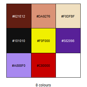
view_palette(all_cols)

Trim colours

Implement a very sketchy way of trimming the colours, by removing similar colours based on a threshold value
Compute the distance matrix for the colours extracted from the image
- Make the diagonal infinity (so it will never be below threshold)
Iterate through the colours removing colours that are within a distance threshold of the current iteration
- This makes the order of both the iteration and the colours important

d <- cols_df %>% dist(method = "maximum")
m <- as.matrix(d)
diag(m) <- Inf

# Set a threshold value
threshold <- 22

# Loop through each column of matrix and remove columns that are a similar colour
# to the current colour (based on threshold)
for(j in colnames(m)){
  if(!(j %in% colnames(m))){next}
  remove <- names(m[,j][m[,j] < threshold])
  if(all(!remove %in% colnames(m))){next}
  m <- m[, -which(colnames(m) %in% remove)]
}

View the trimmed colours

trimmed_cols <- all_cols[colnames(m) %>% as.integer()]
view_palette(trimmed_cols)

Map the closest colour in the image back to the trimmed colours
This should mean that the final colours contained in the palette are actual colours contained within the original image

trimmed_cols <-
  trimmed_cols %>%
  matrix() %>%
  image_read() %>%
  image_map(i) %>%
  image_raster() %>%
  pull(col)

view_palette(trimmed_cols)

Finally, order the trimmed colours based on their frequency in the original image

trimmed_cols_in_order <-
  i %>% 
  image_map(image_read(matrix(c(trimmed_cols, "transparent")))) %>% 
  image_raster() %>% 
  filter(col != "transparent") %>% 
  count(col) %>% 
  arrange(desc(n)) %>% 
  pull(col)

view_palette(trimmed_cols_in_order)

Visualise the image, the palette, and the image made only from the colours in the palette

# Return a visual summary
patchwork::wrap_plots(
  
  # Plot original
  image_ggplot(i) + 
    labs(subtitle = "Original")+
    theme(plot.subtitle = element_text(hjust = 0.5)),
  
  # Plot palette
  view_palette(trimmed_cols_in_order)+
    labs(subtitle = "Palette")+
    theme(plot.subtitle = element_text(hjust = 0.5)),
  
  # Plot image made from the palette
  i %>% 
    image_map(image_read(matrix(c(trimmed_cols_in_order, "transparent")))) %>% 
    image_ggplot() +
    labs(subtitle = "From palette")+
    theme(plot.subtitle = element_text(hjust = 0.5))
)

Function

Wrap the essence of the code above into a function

make_palette <- function(img, threshold = 28, max_cols = 25, dist_method = "maximum"){
  
  # Read image
  i_original <- image_read(img)
  
  # Make image smaller if it's big - as dist() and clustering will only be possible
  # on very small images. Use image_sample to keep original colours in resizing
  if(image_info(i_original)$width > 100){
    i <- i_original %>% image_sample(geometry = "100x")
  } else {
    i <- i_original
  }
  
  # Convert to raster and compute LAB values
  ir <-
    i %>% 
    image_raster() %>%
    as_tibble() %>% 
    filter(col != "transparent") %>% 
    transmute(col2rgb(col) %>% 
                t() %>% 
                farver::convert_colour(from = "rgb", to = "lab") %>% 
                as_tibble())
    
  # Compute distances and hierarchical cluster
  clusts <- dist(ir, method = dist_method) %>% hclust(method = "complete")
  
  # Compute colours from clusters
  cols_df <-
    ir %>%
    mutate(group = cutree(clusts, max_cols)) %>%
    group_by(group) %>%
    summarise(across(c(l,a,b), mean), .groups = "drop") %>%
    select(-group)
  
  # All colours (max_cols) before trimming
  all_cols <- cols_df %>% farver::encode_colour(from = "lab")
  
  # Convert selected colours back to LAB and compute distances
  # Convert distances to matrix and make diagonal Infinity
  d <- cols_df %>% dist(method = dist_method)
  m <- as.matrix(d)
  diag(m) <- Inf

  # Loop through each column of matrix and remove columns that are a similar colour
  # to the current colour (based on threshold)
  for(j in colnames(m)){
    if(!(j %in% colnames(m))){next}
    remove <- names(m[,j][m[,j] < threshold])
    if(all(!remove %in% colnames(m))){next}
    m <- m[, -which(colnames(m) %in% remove)]
  }
  
  # Trim the colours and map colours from the original image to them
  # This should mean the colours in the final palette are colours contained in the original image
  trimmed_cols <- 
    all_cols[colnames(m) %>% as.integer()] %>% 
    matrix() %>%
    image_read() %>%
    image_map(i) %>%
    image_raster() %>%
    pull(col)
  
  # Order the trimmed colours based on how often they appar when mapped onto 
  # the original image
  trimmed_cols_in_order <-
    i %>% 
      image_map(image_read(matrix(c(trimmed_cols, "transparent")))) %>% 
      image_raster() %>% 
      filter(col != "transparent") %>% 
      count(col) %>% 
      arrange(desc(n)) %>% 
      pull(col)
  
  # Return a visual summary
  patchwork::wrap_plots(
    
    # Plot original
    image_ggplot(i_original) + 
      labs(subtitle = "Original")+
      theme(plot.subtitle = element_text(hjust = 0.5)),
    
    # Plot palette
    view_palette(trimmed_cols_in_order)+
      labs(subtitle = "Palette")+
      theme(plot.subtitle = element_text(hjust = 0.5)),
    
    # Plot image made from the palette
    i_original %>% 
      image_map(image_read(matrix(c(trimmed_cols_in_order, "transparent")))) %>% 
      image_ggplot() +
      labs(subtitle = "From palette")+
      theme(plot.subtitle = element_text(hjust = 0.5))
  )
  
}

Run on sprites

Run the function on all sprites with default values
I think these sprites have less than 25 colours (the default cols_max value I chose) - so its really just the colour trimming choosing the palettes on these examples

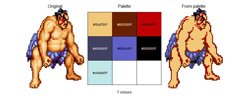
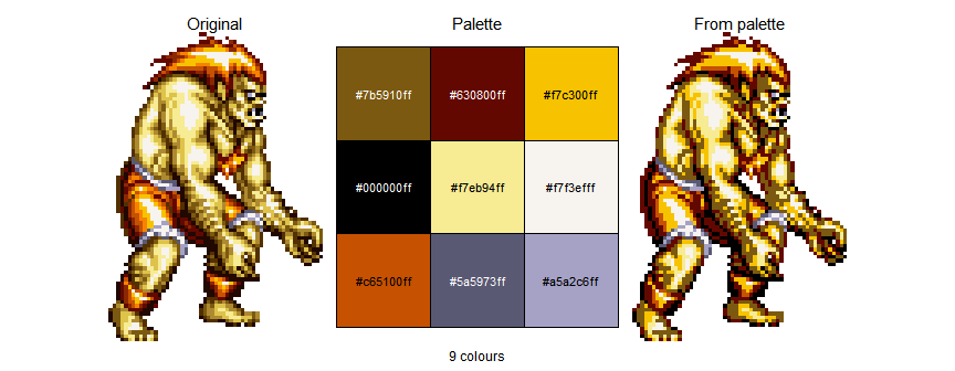
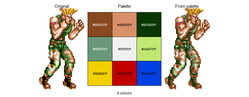
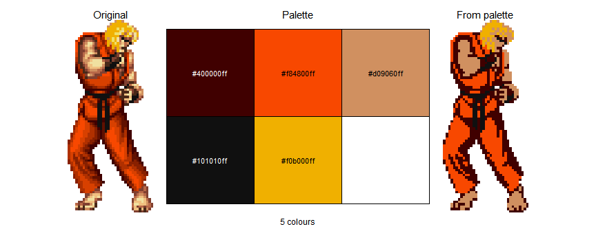
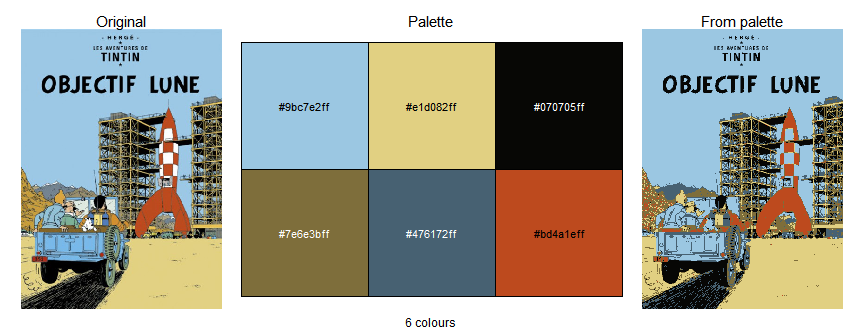
make_palette('files/ryu.png')

make_palette('files/ehonda.png')

make_palette('files/blanka.png')

make_palette('files/guile.png')

make_palette('files/ken.png')

make_palette('files/chun-li.png')

make_palette('files/zangief.png')

make_palette('files/dhalsim.png')

make_palette('files/balrog.png')

make_palette('files/vega.png')

make_palette('files/sagat.png')

make_palette('files/bison.png')

make_palette('files/cammy.png')

make_palette('files/deejay.png')

make_palette('files/fei-long.png')

make_palette('files/t-hawk.png')

Image examples

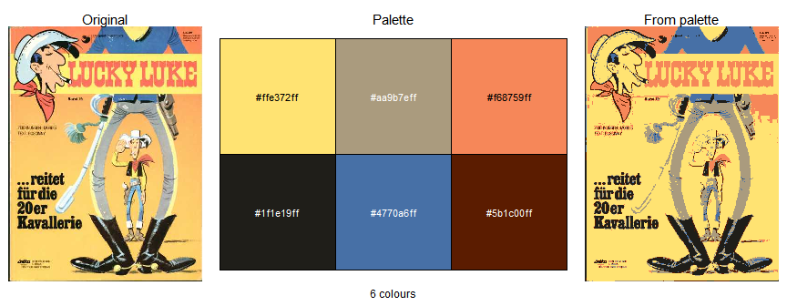
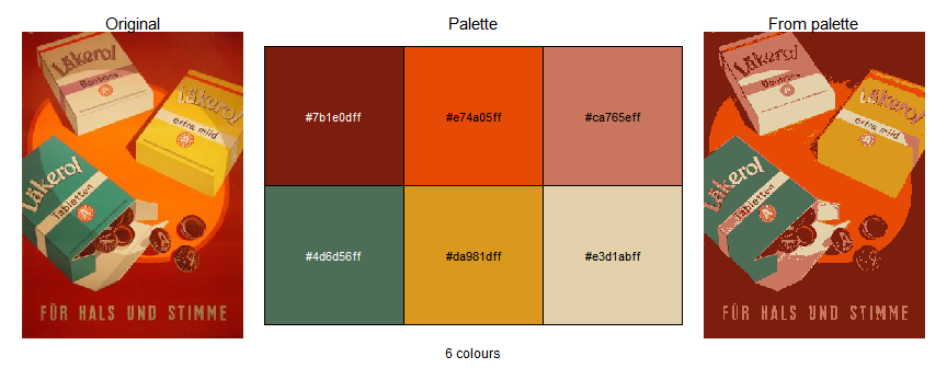
Here I compare the output of my code with some of the example colour palettes created in the {colorfindr} package readme file

make_palette('https://www.movieart.ch/bilder_xl/tintin-et-milou-poster-11438_0_xl.jpg')

make_palette('http://www.coverbrowser.com/image/lucky-luke/5-1.jpg')

make_palette('http://www.gallery29.ie/images/posters/1171469398_DSC03889.jpg')

cj-holmes/ssf2turbo

sf2turbo

Intro

Approach

Function to visualise colours

Read image

Extract colours

Trim colours

Function

Run on sprites

Image examples