The code for this step is contained in the sixth code cell of the IPython notebook located in "advanced_lane_finding.ipynb" in the Camera_Calibration class.
I start by preparing "object points", which will be the (x, y, z) coordinates of the chessboard corners in the world. Here I am assuming the chessboard is fixed on the (x, y) plane at z=0, such that the object points are the same for each calibration image. Thus, objp is just a replicated array of coordinates, and objpoints will be appended with a copy of it every time I successfully detect all chessboard corners in a test image. imgpoints will be appended with the (x, y) pixel position of each of the corners in the image plane with each successful chessboard detection.
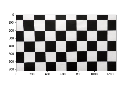
I then used the output objpoints and imgpoints to compute the camera calibration and distortion coefficients using the cv2.calibrateCamera() function. I applied this distortion correction to the test image using the cv2.undistort() function and obtained this result:
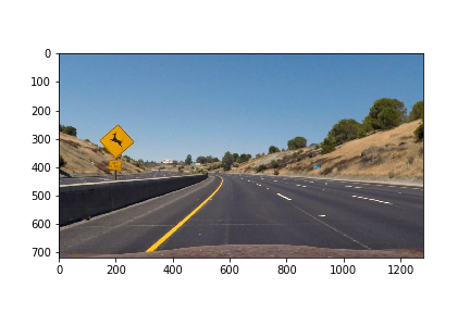
To demonstrate this step, I will describe how I apply the distortion correction to one of the test images like this one:
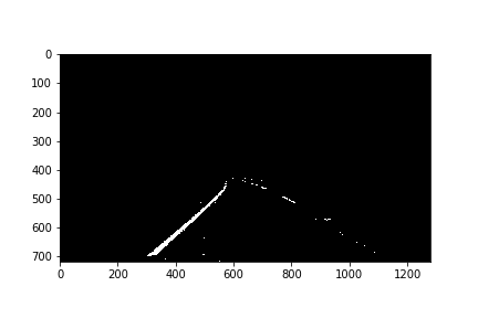
I used a combination of color and gradient thresholds to generate a binary image. The code for this is contained in the apply_threshold function. Here's an example of the output for this step.
The code for my perspective transform includes a function called transform_perspective. After manually analyzing the test inputs, I chose the hardcode the source and destination points in the following manner:
| Source | Destination |
|---|---|
| 382, 600 | 441, 600 |
| 500, 517 | 441,517 |
| 922, 600 | 857, 600 |
| 793, 517 | 857, 517 |
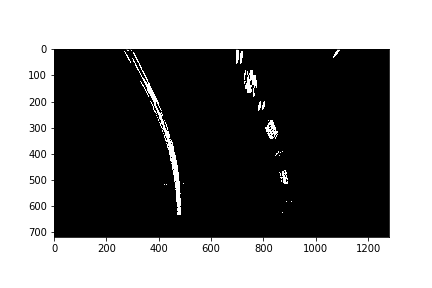
I verified that my perspective transform was working as expected by drawing the src and dst points onto a test image and its warped counterpart to verify that the lines appear parallel in the warped image.
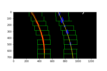
Then I used a sliding window histgram to find high itensity points in the binary image, and fit my lane lines with a 2nd order polynomial kinda like this:
This is in the calculate method of the Line class.
5. Calculate the radius of curvature of the lane and the position of the vehicle with respect to center.
This was done in the __find_radius_of_curvature method in the Line class.
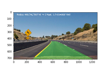
Finally, in the unwarp function, I applied the inverse perspective transform and annotated the image with the radius of curvature, center offset, and lane lines.
Here's a link to my video result
I faced signifant challenges with shadows and lighting. Optimizing the gradient and s channel thresholds helped in this area. Filtering out undesirable images was also helpful. To make it more robust, more optimization can be done in the selection of the color space and thresholds. Another possible improvement would be to use the record of polynomial fits to find a rate of change in fits from frame to frame, and reject rapid changes.
