Tensor flow project. Takes in images of traffic signs and classifies them.
The pandas library was used to calculate summary statistics of the traffic signs data set:
- The size of training set is 34799
- The size of the validation set is 4410
- The size of test set is 12630
- The shape of a traffic sign image is 32 x 32 x 3
- The number of unique classes/labels in the data set is 43
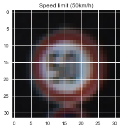
This is a typical example of one of the images in the data sets
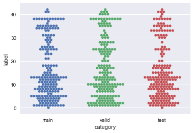
The following is a swamrmplot of the validation, test, and training data sets. It shows the distribution of the data by traffic sign type.

Before training the model with the image data, each image was preprocessed so that each pixel had approximately zero mean and equal variance. This reduces the work the optimizer has to do and leads to higher validation accuracy.
The final model consisted of the following layers:
| Layer | Description |
|---|---|
| Input | 32x32x3 RGB image |
| Convolution 5x5 | 1x1 stride, valid padding, outputs 28x28x6 |
| RELU | |
| Max pooling | 2x2 stride, outputs 14x14x6 |
| Convolution 5x5 | 1x1 stride, valid padding, outputs 10x10x16 |
| RELU | |
| Max pooling | 2x2 stride, outputs 5x5x16 |
| Flatten | outputs 400 |
| Fully connected | outputs 120 |
| RELU | |
| Fully connected | outputs 84 |
| RELU | |
| Dropout | keep probabiliy of 50% |
| Fully connected | outputs 43 |
| Softmax |
To train the model, TensorFlow's AdamOptimizer was used to reduce the softmax cross entropy between the training data and one-hot encoded labels. It was found that with a learning rate of 0.002, 10 epochs was sufficient to achieve a validation accuracy of around 95%. I used a Batch size of 128.
My final model results were:
- Validation set accuracy of 0.957
- Test set accuracy of 0.917
The initial architecture was LeNet. It was chosen because it has a record of good performance, and it has been used sucessfully in handwriting recognition with MNIST data. It includes multliple convolution layers, which help the model to be spatially independent. Translation independance is a key feature for succesful traffic sign cliassfication.
I wasn't able to get a satisfactory validation accuracy with the LetNet architecture, so dropout was added in between the last two fully connected layers. Dropout substantially improved the validation acuracy by reducing overfitting on the training set. After adding dropout, I course-tuned the learning rate in a logarithmic progression. When I found the order of magnitude with the best performance, I fine-tuned the learning rate to establish the choice I made. Accuracy gains diminished after 10 epochs, so this number of epochs was chosen.
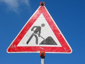
Here are five German traffic signs that I found on the web:
The first image is likely to be easy to classify, since all of the characteristics of the sign are evident without artifacts. The third image has details that are small enough to be lost when the image is reduced to 32 x 32 pixels. The fourth image might be difficult to classify because of the distortion of its shape caused by the image angle.
Here are the results of the prediction:
| Image | Prediction |
|---|---|
| No entry | No entry |
| Speed limit (30km/h) | Speed limit (30km/h) |
| Road work | Road work |
| Stop | Stop |
| Yield | Yield |
The model was able to correctly guess 5 of the 5 traffic signs, which gives an accuracy of 100%. This compares favorably to the accuracy on the test set of 0.917.
For the first image, the model is basically completely sure that it is a no entry sign. Given the pristine nature of the image, this is not surprising.
| Probability | Prediction |
|---|---|
| 1.0 | No entry |
| 1.55949e-18 | Stop |
| 1.24926e-29 | Traffic signals |
| 2.52315e-30 | Speed limit (20km/h) |
| 1.56718e-32 | No passing |
For the second image, more uncertainty was observed. The probability for the correct label was barely greater than the one for 60km.
Speed limit (30km/h) Speed limit (60km/h) Speed limit (80km/h) Speed limit (50km/h)
| Probability | Prediction |
|---|---|
| 0.484122 | Speed limit (30km/h |
| 0.45101 | Speed limit (60km/h |
| 0.0646315 | Speed limit (80km/h |
| 0.000235438 | Speed limit (50km/h |
| 1.35486e-07 | Dangerous curve to the right |
For the third image, it is again quite certain. Surprisingly so, given concerns about pixel resolution
| Probability | Prediction |
|---|---|
| 0.984733 | Road work |
| 0.0150242 | Beware of ice/snow |
| 0.000119586 | Road narrows on the right |
| 7.56106e-05 | Slippery road |
| 4.05349e-05 | Double curve |
Another surprise in the fourth image. The shape distortion does not appear to have confused the model.
| Probability | Prediction |
|---|---|
| 0.999996 | Stop |
| 2.85719e-06 | No entry |
| 0.000119586 | Road work |
| 8.92196e-09 | No passing for vehicles over 3.5 metric tons |
| 8.61496e-09 | Speed limit (80km/h) |
Very high certainty for the final image also. This image is also relatively artifact free.
| Probability | Prediction |
|---|---|
| 1.0 | Yield |
| 1.37867e-08 | Speed limit (80km/h) |
| 6.58397e-10 | Speed limit (60km/h) |
| 3.79426e-11 | Road work |
| 2.40711e-12 | Speed limit (50km/h) |


