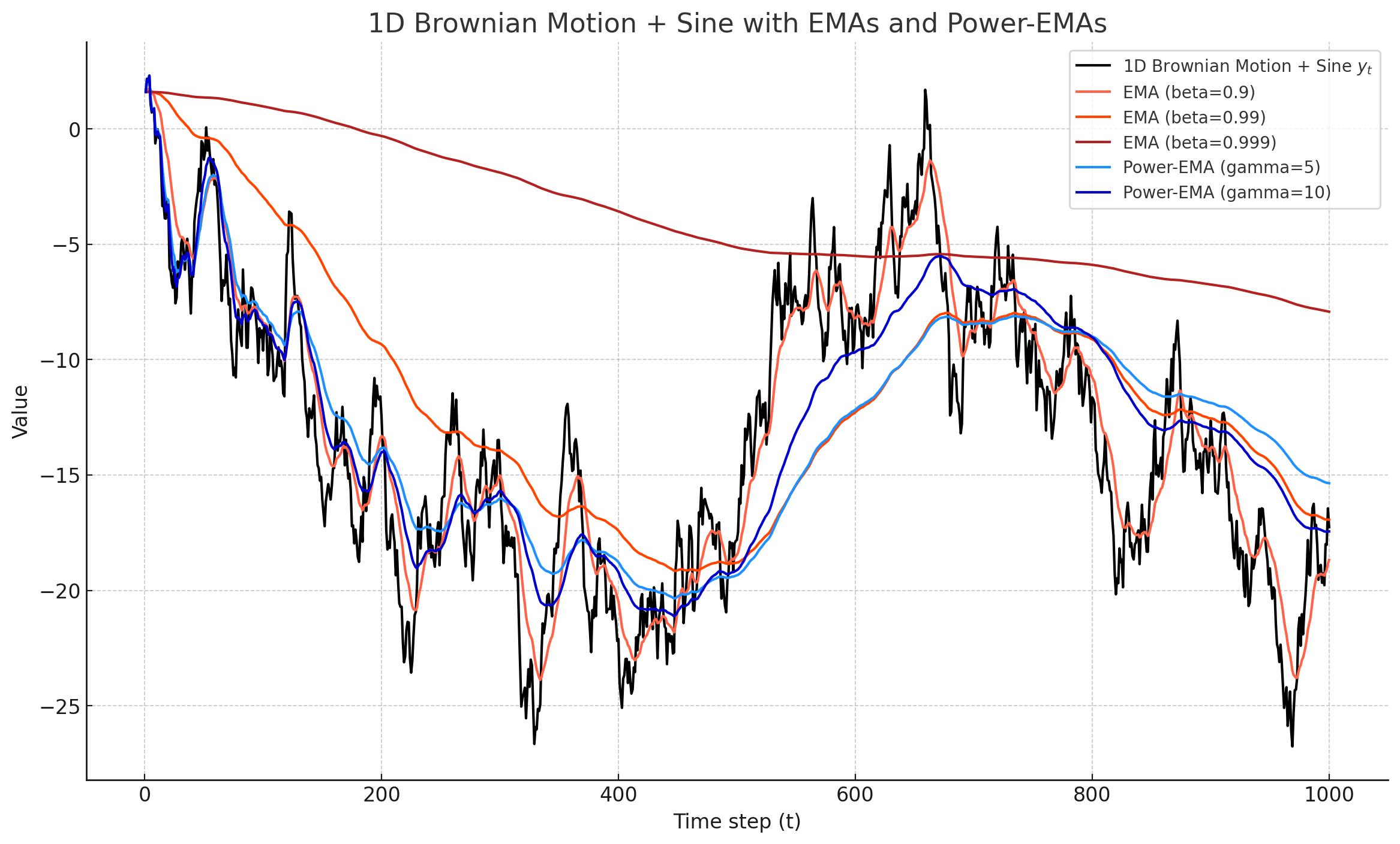
Karras Power Function EMA (Post-training EMA synthesis)

This tutorial-repo implements the Karras's Power function EMA, quite incredible trick introduced in the paper Analyzing and Improving the Training Dynamics of Diffusion Models by Tero Karras, Miika Aittala, Jaakko Lehtinen, Janne Hellsten, Timo Aila, Samuli Laine.

So What is Karras's Power function EMA?

I recommend you to read the paper for full detail, but here is the big picture.

Recall that EMA'ing checkpoint is about keeping track of smooth-version of model parameters, $\theta_\beta$, where $\theta_\beta(t) = \beta \theta_\beta(t-1) + (1-\beta) \theta(t)$

, where $\beta$ is the decaying factor close to 1. Using EMA typically makes the model more robust, and it is a common practice in training deep neural networks.

You want to use EMA, but...

You don't want the ema to be too slow, because it will make random initialization's contribution to the final model too big.
You definitely want the decaying factor to be self-similar, because you should be able to increase-time of the training.
You want to set decaying factor post-hoc, because you don't want to retrain the model from scratch with different decaying factor.

Karras's Power function EMA is the answer to all of these problems. He first uses power-function version of EMA where instead of keeping beta constant, he uses $\beta(t) = (1 - 1/t)^{1 + \gamma}$, where $\gamma$ is the hyperparameter. This makes the contribution of historical parameters self-similar, and you can increase the time of the training and it will not change how you expect the EMA to behave (i.e., if you want first 10% of the training to contribute x% of the final model, increasing/decreasing training time will not change that).

Overall Algorithm and Implementation

So there is two main part of the algorithm.

Saving two copies of the EMA-model, each with different width.
Recovering arbitrary-width EMA

Think of width as decaying factor. Larger width means it will be smoother.

First, save two copies of the EMA, with different width

This is the easy part. You just need to save two copies of the EMA, each with different width (different $\gamma$).

gamma_1 = 5
gamma_2 = 10
model = Model()
model_ema_1 = copy.deepcopy(model).cpu()
model_ema_2 = copy.deepcopy(model).cpu()


for i, batch in enumerate(data_loader):
    beta_1 = (1 - 1/(i+1)) ** (1 + gamma_1)
    beta_2 = (1 - 1/(i+1)) ** (1 + gamma_2)
    # train model
    loss.backward()
    optimizer.step()
    for p, p_ema_1, p_ema_2 in zip(model.parameters(), model_ema_1.parameters(), model_ema_2.parameters()):
        p_ema_1.data = p_ema_1.data * beta_1 + p.data * (1 - beta_1)
        p_ema_2.data = p_ema_2.data * beta_2 + p.data * (1 - beta_2)
    
    if i % save_freq == 0:
        torch.save(model_ema_1.state_dict(), f'./model_ema_1_{i}.pth')
        torch.save(model_ema_2.state_dict(), f'./model_ema_2_{i}.pth')

Second, recover arbitrary-decay EMA after training.

Now what if you want to recover EMA with $\gamma_3$? Incredibly, you can do this with all the saved checkpoints. The math behind this in the paper is bit... not straightforward so here is my version of the explanation.

EMA, by definition, can be considered as integral of trajectory of the model parameters. So if you have some weighting function $w(t)$, such that

$$\theta_e(T) = \int_0^t w(t) \theta(t) dt$$

For a fixed training runs, $t \in [0, T]$, because we saved two copies of EMA for every, say, total of $n$ checkpoints for different $\gamma$ this means we know the integral value of the trajectory of the

$$\theta_{i,j} = \int_0^T w_{i, j}(t) \theta(t) dt$$

for $i = 1, 2$ and $j = 1, 2, \cdots, n$. $i$ correponds to different width, $j$ corresponds to $j$ th checkpoint. Notice how

$$ w_{i, j}(t) = \begin{cases} t^{\gamma_i} / g_{i,j} & \text{if } t < j \\ 0 & \text{otherwise} \end{cases} $$

where $g_{i,j}$ is simply the normalization constant to make $\int_0^T w_{i, j}(t) dt = 1$.

Our goal is then to

find a approximate $\hat{w}_3(t)$ that will give us the EMA that corresponds with $\gamma_3$.
find the correpsonding $\theta_{3,T}$

See where this is going? Our goal is to approximate $w_3(t)$ as linear combination of $w_{1, j}(t)$ and $w_{2, j}(t)$, i.e.,

$$w_3(t) = \sum_{j=1}^n \alpha_j w_{1, j}(t) + \beta_j w_{2, j}(t)$$

where $\alpha_j$ and $\beta_j$ are the coefficients we need to find. This way,

$$\theta_{3,T} = \int_0^T w_3(t) \theta(t) dt = \sum_{j=1}^n \alpha_j \theta_{1, j} + \beta_j \theta_{2, j}$$

Aha! Now we can find $\alpha_j$ and $\beta_j$ by solving the linear system of equations. Let's just take this one step further.

Goal let us project $w_3(t)$ onto the subspace spanned by $w_{1, j}(t)$ and $w_{2, j}(t)$

We have $K$ functions $f_k(t)$, we have a target $g(t)$ and we want to find $k$ coefficients $\alpha_i$ such that

$$\min \int_0^T \left( g(t) - \sum_{i=1}^K \alpha_i f_i(t) \right)^2 dt$$

How would you solve this?

Define inner product as

$$\langle f, g \rangle = \int_0^T f(t) g(t) dt$$

Then we can rewrite the problem as

$$\min \left | g - \sum_{i=1}^K \alpha_i f_i \right |_2^2$$

if we define $| f |_2 = \sqrt{\langle f, f \rangle}$, expanding the norm, we get

$$\min {\left \| g \right \|_2}^2 - 2 \sum_{i=1}^K \alpha_i \langle g, f_i \rangle + \sum_{i=1}^K \sum_{j=1}^K \alpha_i \alpha_j \langle f_i, f_j \rangle$$

Ha, so substituting $A_{i,j} = \langle f_i, f_j \rangle$ and $b_i = \langle g, f_i \rangle$, we actually just had linear least square problem!

$$\min \left | g \right |_2^2 - 2 \alpha^T b + \alpha^T A \alpha$$

where $\alpha = (\alpha_1, \cdots, \alpha_K)^T$.

So the solution is simply

$$\alpha = A^{+} b$$

where $A^{+}$ is the pseudo-inverse of $A$. We are left to just use the $\alpha$ to get $\theta_{3,T}$.

Note : Well if you ever studied functional analysis, you realize hey, there exists unique solution to this problem, via Hilbert's Projection Theorem. The above is simply finding the projection of $g$ onto the subspace spanned by $f_i$, in $L^2$ space.

So thing you learned:

The level of approximation is determined by the number of checkpoints you saved. More checkpoints, better approximation.
This doesn't have to be power-function EMA. You can use any weighting function $w(t)$, as long as you can compute the integral of the trajectory of the model parameters.

I don't care about the math just give me the code?

Ok, but reminder this is just for a power-function EMA. You can use this for any weighting function $w(t)$.

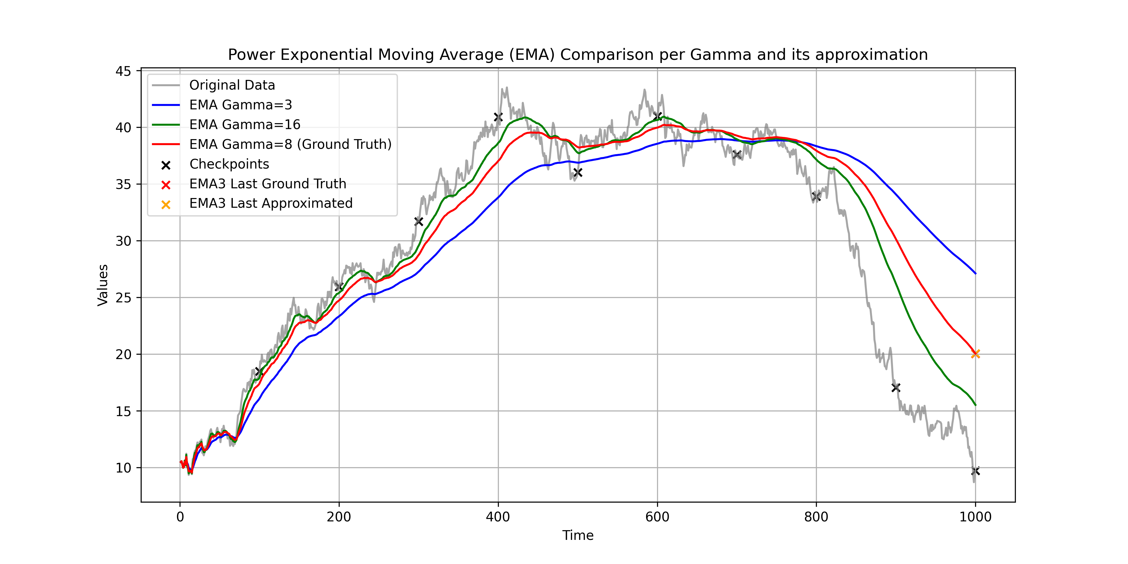
In the above code, you saved two copies of EMA, each with different $\gamma$. Now you want to recover EMA with $\gamma_3$. Suppose you saved $n$ checkpoints, at iteration $i_1, i_2, \cdots, i_n$. Then you can do the following.

t_checkpoint = t[checkpoint_index]
    
ts = np.concatenate((t_checkpoint, t_checkpoint))
gammas = np.concatenate(
    (
        np.ones_like(checkpoint_index) * gamma_1,
        np.ones_like(checkpoint_index) * gamma_2,
    )
)

x = solve_weights(ts, gammas, last_index, gamma_3)
emapoints = np.concatenate((y_t_ema1[checkpoint_index], y_t_ema2[checkpoint_index]))

y_t_ema3 = np.dot(x, emapoints)

where solve_weights is the function that solves the linear least square problem. You can find the implementation in ema_eq.py.

The result is the EMA with $\gamma_3$.