bayesid

Tools for Bayesian system identification.

bayesid delivers methods for System Identification using Bayesian neural networks with nonparametric noise processes [1]. Additionally, a autoregressive Bayesian neural network similar to [2] is implemented.

Dependencies

It is assumed that the user has or is able to install julia. This project has been developed in julia v1.7.1. The R package TimeSeries.OBeu is are also required for some functions used for plotting to work as expected.

Code structure

The core files regarding the methods illustrated in [1] are located in src folder. Subfolders mcmc and models contain code for the Hamiltonian Monte Carlo sampler [*] and structs to implement neural networks using Flux, similar to neural networks implemented at Pkg DiffEqFlux.jl.

Scripts for simulating the logistic data as well as the real data used in the paper are located in data folder.

The folder examples contains simple scripts for running the sampler on data from data folder.

[*] hmc.jl is based on an implementation in SGMCMC.jl--see src/mcmc/LICENSE.

Environment activation

In order to install all dependencies in the current state, start julia from the location bayesid is downloaded. The project folder contains Manifest.toml and Project.toml files so you can type in the REPL

julia> ]
(@v1.7) pkg> activate .
(bayesid)> instantiate

This will make julia install all the necessary packages and dependencies for the available functions.

An example

Having completed the installation process we can run an example by first loading necessary packages and files

using Plots, Random, Distributions, Flux, Zygote, LinearAlgebra
using StatsBase, StatsPlots, KernelDensity, DelimitedFiles, LaTeXStrings
using Parameters: @with_kw
include("../src/models/bnn.jl")
include("../src/mcmc/hmc.jl")
include("../src/utils.jl")
include("../src/npbnn.jl")
include("../src/arbnn.jl")
include("../src/plottools.jl")
include("../src/R/RUtils.jl")

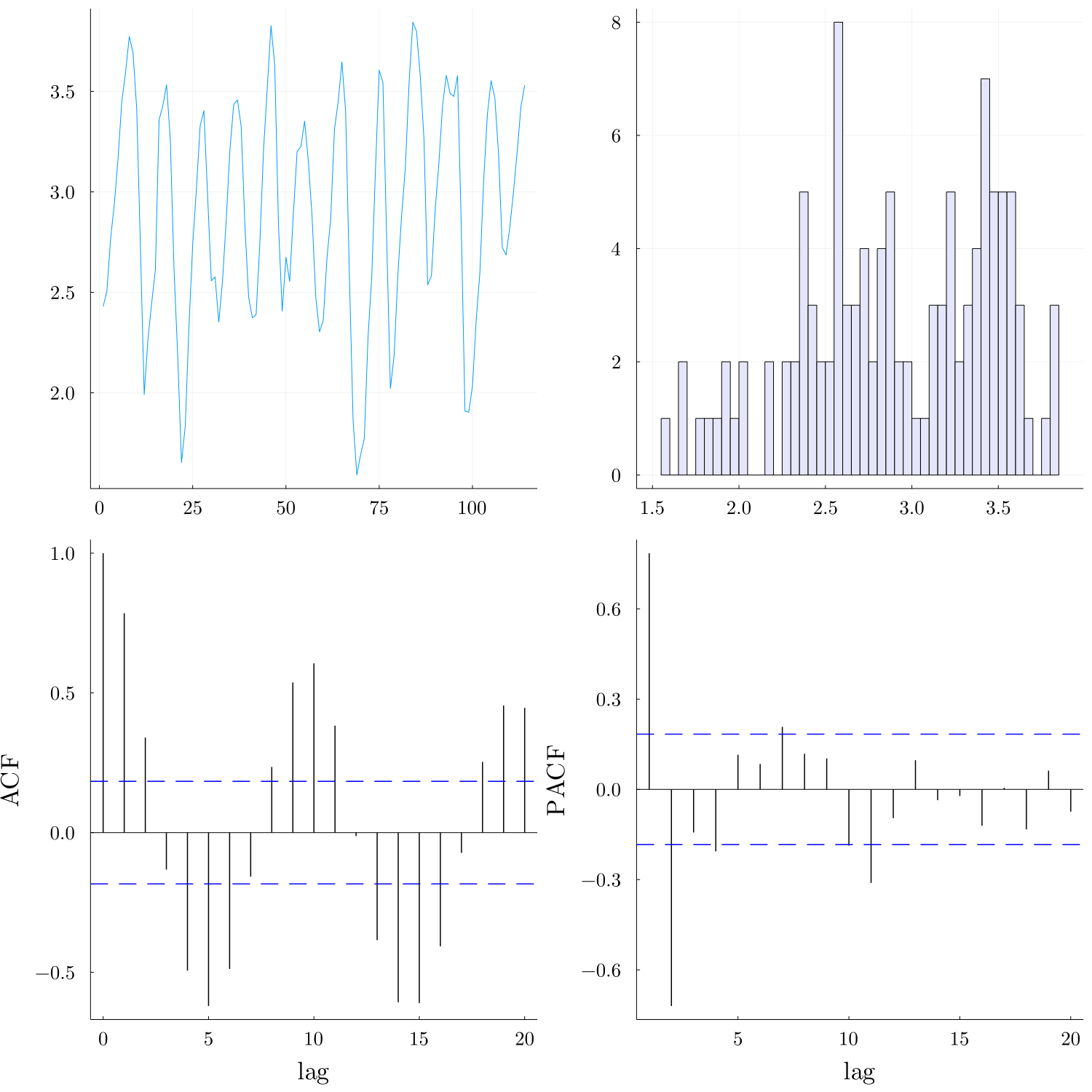
Next, we load the data and explore the time series along with the ACF and PACF.

data = log.(10, readdlm("./data/lynx.txt"));
data_plot = explore_data(data) # requires Rs TimeSeries.OBeu and ts

The PACF plot show significant partial autocorrelations at lags 1,2. Assuming that the data are coming from order 2 Markovian process, we construct the delayed time series

# split training data first 100 observations and generate the lagged time series via embed
lag = 2;
ytemp = data[1:end-14];
D = embed(ytemp, lag+1);

# train data
ytrain = convert(Array{Float64, 2}, hcat(D[:, 1]...));
xtrain = convert(Array{Float64, 2}, D[:, 2:end]');
ytest = data[101:end];

Finally, a neural network is defined and a mutable struct containing the model and HMC parameters specification is defined. We identify the system using the npbnn function.

@with_kw mutable struct Args
    net = g
    maxiter = 40000 # maximum number of iterations
    burnin = 20000 # burnin iterations
    x = xtrain # lagged data
    y = ytrain
    geop = 0.5
    hyper_taus = [1. 1. ;1. 1.]
    ap = 1. # beta hyperparameter alpha for the geometric probability
    bp = 1. # beta hyperparameter beta for the geometric probability
    at = 0.05 # atoms  gamma hyperparameter alpha
    bt = 0.05 # atoms gamma hyperparameter beta
    ataus = 5ones(2,2) # Gamma hyperprior on network weights precision
    btaus = 5ones(2,2) # IG hyperprior on network weights precision
    seed = 123
    stepsize = 0.005
    numsteps = 20
    verb = 1000
    npredict = 14
    save = false
    filename = "/sims/lynx/npbnn/"
end
@time est = npbnn();

More details can be found in the /examples/canadianlynx.jl file.

Parametric models

We have included some state-of-the-art parametric models like ARMA based on R, using Julia's interoperability. These are in src/R/RUtils.jl

References

[1] Merkatas, C., & Särkkä, S. (2022). System identification using autoregressive Bayesian neural networks with nonparametric noise processes. Journal of Time Series Analysis.

[2] Nakada, Y., Matsumoto, T., Kurihara, T., & Yosui, K. (2005). Bayesian reconstructions and predictions of nonlinear dynamical systems via the hybrid Monte Carlo scheme. Signal processing, 85(1), 129-145.