PyPegase 0.1

Introduction

PyPegase provides a convenient way to generate galaxy models using the PEGASE version 2 code. It provides a wrapper class that encapsulates the parameters to, and results from the PEGASE binaries. This makes it much simpler to explore the paramater space and examine the outputs from the resulting models.

PyPegase assumes you have a clean installation of the PEGASE2 code, and have compiled the Fortran sources to produce executable binaries called SSPs, scenarios, spectra, calib and colors.

For more on PEGASE see the docs: http://arxiv.org/abs/astro-ph/9912179

Installation and configuration

If you use pip, install with:

pip install pypegase

alternatively, get from github:

git clone https://github.com/coljac/pypegase.git

and add the directory to your PYTHONPATH environment variable.

You will also need to point PyPegase to your PEGASE2 directory, the location of the binaries (such as SSPs, etc). The best way to do this is with a PEGASE_HOME environment variable, but can be done at runtime by setting PEGASE.pegase_dir = "<path to PEGASE>".

You can also create a .pypegase file to override the module's defaults - see defaults below.

Usage

Usage of PyPegase is centred on the PEGASE class which encapsulates a run of the PEGASE code. Other classes such as IMF, SSP, SFR and Scenario wrap the inputs to the PEGASE code, though use of these is in most cases optional.

The basic workflow is as follows:

Create an IMF object for your model (optional)
Create an SSP object with the IMF (optional)
Create one or more Scenario objects (optional)
Create PEGASE instance, passing in the above
Invoke .generate() on the PEGASE object, which generates the data files
Access the results via the colors() and spectra() methods
Save the resulting object with save_to_file() so it can be later loaded with PEGASE.from_file() and save on generation time.

All of this can be done in one line, see the examples below.

Note that all the outputs created by PEGASE end up in the PEGASE home directory.

Defaults

The default values are all as per the PEGASE documentation and code, with the following exceptions:

The default IMF is Salpeter 1955
The default SFR is exponentially decreasing instead of instantaneous burst, with the default values for p1 and p2 as per the code (1000 and 1 respectively).

For convenience, defaults can be overridden by creating a file .pypegase in your home directory. It should have the format:

variable = value
variable2 = value2
...

To see the built-in defaults, execute PEGASE.list_defaults(). You can use this string as a template. To get started, try:

python -c "import pypegase as pp; pp.PEGASE.list_defaults()" > ~/.pypegase

This will create an file for you that you can edit should you wish to override some of the defaults. (Note: If pypegase.py is not in your system's library dir, you will need it in the current directory or you can add the location of pypegase.py to to PYTHONPATH environment variable.)

Spectra and colors

Generated spectra and colors data can be obtained with the spectra() and colors() methods respectively. In each case the result will be an Astropy table.Table with a row for each timestep.

Both of these methods can take a list of columns as the cols parameter. For spectra especially the resulting table is very large and it may make sense to filter the results in this way. The available column names are the wavelengths and spectral lines as they appear in the xxx_spectra.dat file as well as the following:

time m_gal m_star m_wd m_nsbh m_substellar m_gas z_ism z_stars_mass
z_stars_bl l_bol od_v l_dust_l_bol sfr phot_lyman rate_snii rate_snia
age_star_mass age_star_lbol

Note that column names must match PEGASE's file output exactly - so for instance "100200." will work, but "100200" will not.

The available column names can be viewed with peg_instance.spectra().colnames() (and the same for colors).

The table returned by these methods can be further filtered with the time_lower and time_upper keywords; for example, to return only rows with a time between 100 and 13000 Myr, call colors(time_lower=100, time_upper=13e3).

These methods return a table which can be accessed as mytable['colname'] (returns entire column) or mytable['colname'][n] (returns column _colname_ at row _n_).

Examples

Generate a set of data using the defaults, in files prefixed with mydata_:

from pypegase import *
import matplotlib.pyplot as plt

PEGASE.pegase_dir = '/home/me/PEGASE.2/' # unless PEGASE_HOME is set

peg = PEGASE('mydata') # default IMF, Scenario, etc
peg.generate() # some minutes may be required, console will show progress
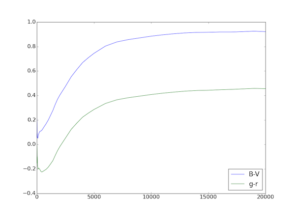
colors = peg.colors()
colors['B-V'][-1] # B-V color at last timestep (20 Gyr) = .922
plt.plot(colors['time'], colors['B-V']) # plot times versus B-V color
plt.plot(colors['time'], colors['B-V'], "b-", label="B-V") # plot times versus B-V color
plt.plot(colors['time'], colors['g-r'], "g-", label="g-r")
plt.legend(loc = 'lower right', numpoints=1)

peg.save_to_file(peg.name + '.peg')

peg2 = PEGASE.from_file(peg.name + '.peg')
peg2.colors() # Same as above

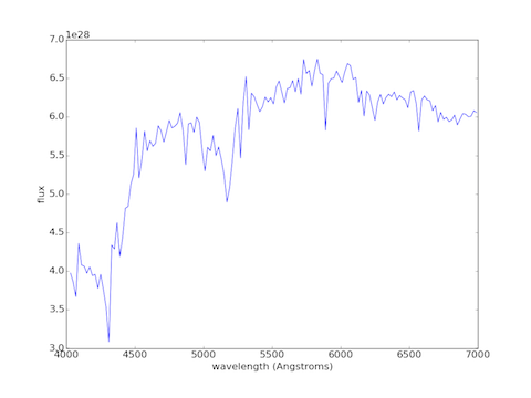
Plotting a continuum spectrum at t=13000 Myr:

peg = ... # one I made earlier with defaults
spectra = peg.spectra(time_lower=13000, time_upper=13000)
lambdas = []
vals = []
filters = (4010, 7010) # lower, upper wavelengths (roughly V)
for col in spectra.colnames:
    try:
        l = float(col)
        if l > filters[0] and l < filters[1]:
            lambdas.append(l)
            vals.append(spectra[col][0])
    except ValueError:
        pass # Column is not a number (i.e. wavelength)
plot(lambdas[:149], vals[:149], "b-") # Removed the lines for this example
xlabel("wavelength (Angstroms)")
ylabel("flux")

Specifying parameters explicitly (these are all the default values and any can be omitted):

peg = PEGASE("custom", ssps=SSP(
    IMF(IMF.IMF_Salpeter), ejecta=SNII_ejecta.MODEL_B, winds=True
), scenario=Scenario(
    binaries_fraction=0.04, metallicity_ism_0=0, infall=False, sfr=SFR(SFR.EXPONENTIAL_DECREASE, p1=1e3, p2=1),
    metallicity_evolution=True, substellar_fraction=0, winds=False, neb_emission=True,
    extinction=Extinction.NO_EXTINCTION
))
peg.generate()
spec = peg.spectra(cols=['time', 'l_bol', '7135.00'])
spec['l_bol'][20] # == 2.499E34

Experimenting with IMFs:

# Built-in
imf = IMF(IMF.IMF_Scalo86)
imf = IMF(IMF.IMF_MillerScalo) # and so on for built-in IMFs

# Custom
imf = IMF(IMF.CUSTOM, lower_mass=0.1, upper_mass=120, gamma=-1.35) # A custom IMF equivalent to Salpeter with
                                                                   # default cutoffs
imf = IMF(IMF.CUSTOM, lower_mass=0.1, upper_mass=120, powers=[
    (0.1, -0.4),
    (1., -1.5),
    (10., -2.3)
]) # A custom IMF equivalent to Miller-Scalo (see IMF_MillerScalo.dat)

peg = PEGASE("custom_imf", ssps=SSP(imf))

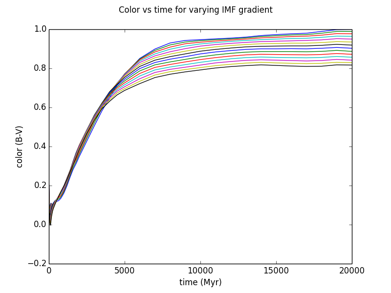
Generating a series of models with varying parameters:

pegase = PEGASE('test')
for gamma in np.arange(-1.7, -1.0, 0.05):
    # Reuse the same instance each iteration
    pegase.name = "imftest_" + str(gamma)
    pegase.ssps.imf = IMF(IMF.CUSTOM, gamma=gamma)
    pegase.generate()
    pegase.save_to_file(pegase.name + ".peg")

Plotting the results:

pegs = PEGASE.from_dir(".")
# Now we have a list of PEGASE instances

for i, peg in enumerate(pegs):
    colors = peg.colors(cols=['B-V']) # Note 'time' included by default
    plt.plot(colors['time'], colors['B-V'])

plt.suptitle(r'Color vs time for varying IMF gradient')
plt.xlabel('time (Myr)')
plt.ylabel('color (B-V)')
plt.show()

Further work

Future versions will include:

Passing a redshift value into spectra and colors
Custom filters
Calculating colors directly from spectra information
Better ability to handle customised installations of PEGASE, in particular an altered IMF list/timesteps
Ability to instantiate from a dictionary, JSON and other formats
Ability to access color and spectra data by time as well as row number
More intuitive use of multiple scenarios
Ability to specify your own defaults
Simplified process for wrapping an existing run (will examine the file system and reverse-engineer the parameters)
Human-readable pickled (saved) files
Unit tests for a greater variety of scenarios
A more robust copy() implementation
Console GUI

Acknowledgement

PyPegase was written with the support of the Centre for Astrophysics and Supercomputing at Swinburne University of Technology.