GREED : Bayesian greedy clustering

Greed enables model-based clustering of networks, matrices of count data and much more with different types of generative models. Model-selection and clustering are performed in combination by optimizing the Integrated Classification Likelihood. Details of the algorithms and methods proposed by this package can be found in Côme, Jouvin, Latouche, and Bouveyron (2021) 10.1007/s11634-021-00440-z.

Dedicated to clustering and visualization, the package is very general and currently handles the following tasks:

Continuous data clustering with Gaussian Mixture Models. A GMM tutorial is available. See also the documentation for the Gmm and DiagGmm S4 classes.
Graph data clustering with the Stochastic Block Model or its degree corrected variants. A SBM tutorial is available . See also the documentation for the Sbm and dcSbm S4 classes.
Categorical data clustering with the Latent Class Analysis. An LCA tutorial is available. See also the documentation for the Lca S4 class.
Count data clustering with the Mixture of Multinomials model. A tutorial will soon be available. For now, we refer to the documentation for the Mom S4 class.
Mixed-typed data clustering, e.g. categorical and numerical but the package handles virtually any type of data combination by stacking models on top of each data types. For example graph data with continuous or categorical data attached to the nodes are handled. A CombinedModels tutorial is available. See also the documentation for the CombinedModels S4 class.
Mixture of regression for simultaneous clustering and fitting a regression model in each cluster. A MoR tutorial is available. See also the documentation for the MoR S4 class.
Co-clustering of binary and count-data via the Latent Block Model and its degree-corrected variant. A tutorial will soon be available. For now, we refer to the documentation for the DcLbm S4 class.

With the Integrated Classification Likelihood, the parameters of the models are integrated out with a natural regularization effect for complex models. This penalization allows to automatically find a suitable value for the number of clusters K^⋆. A user only needs to provide an initial guess for the number of clusters K, as well as values for the prior parameters (reasonable default values are used if no prior information is given). The default optimization is performed thanks to a combination of a greedy local search and a genetic algorithm described in Côme, Jouvin, Latouche, and Bouveyron (2021), but several other optimization algorithms are also available.

Eventually, a whole hierarchy of solutions from K^⋆ to 1 cluster is extracted. This enables an ordering of the clusters, and the exploration of simpler clustering along the hierarchy. The package also provides some plotting functionality.

Installation

You can install the development version of greed from GitHub with:

#GitHub
install.packages("devtools")
devtools::install_github("comeetie/greed")

Or use the CRAN version:

#CRAN
install.packages("greed")

Usage: the greed function

The main entry point for using the package is simply thegreed function (see ?greed). The generative model will be chosen automatically to fit the type of the provided data, but you may specify another choice with the model argument.

We illustrate its use on a graph clustering example with the classical Books network ?Books.

More use cases and their specific plotting functionality are described in the vignettes.

library(greed)
data(Books)
sol <- greed(Books$X) 
#> 
#> ── Fitting a guess DCSBM model ──
#> 
#> ℹ Initializing a population of 20 solutions.
#> ℹ Generation 1 : best solution with an ICL of -1347 and 3 clusters.
#> ℹ Generation 2 : best solution with an ICL of -1346 and 4 clusters.
#> ℹ Generation 3 : best solution with an ICL of -1346 and 4 clusters.
#> ── Final clustering ──
#> 
#> ── Clustering with a DCSBM model 3 clusters and an ICL of -1345

You may specify the model you want to use and set the priors parameters with the (model argument), the optimization algorithm (alg argument) and the initial number of cluster K. Here Books$X is a square sparse matrix and a graph clustering ?`DcSbm-class` model will be used by default. By default, the Hybrid genetic algorithm is used.

The next example illustrates a usage without default values. A binary Sbm prior is used, along with a spectral clustering algorithm for graphs.

sol <- greed(Books$X,model=Sbm(),alg=Seed(),K=10)
#> 
#> ── Fitting a guess SBM model ──
#> 
#> ── Final clustering ──
#> 
#> ── Clustering with a SBM model 5 clusters and an ICL of -1255

Result analysis

The results of greed() is an S4 class which depends on the model argument (here, an SBM) which comes with readily implemented methods: clustering() to access the estimated partitions, K() the estimated number of clusters, and coef() the (conditional) maximum a posteriori of the model parameters.

table(Books$label,clustering(sol)) %>% knitr::kable()

	1	2	3	4	5
c	0	1	6	36	6
l	8	30	5	0	0
n	0	2	8	3	0

K(sol)
#> [1] 5
coef(sol)
#> $pi
#> [1] 0.07619048 0.31428571 0.18095238 0.37142857 0.05714286
#> 
#> $thetakl
#>             [,1]        [,2]        [,3]        [,4]       [,5]
#> [1,] 0.821428571 0.367424242 0.065789474 0.003205128 0.00000000
#> [2,] 0.367424242 0.106060606 0.006379585 0.003885004 0.00000000
#> [3,] 0.065789474 0.006379585 0.251461988 0.016194332 0.04385965
#> [4,] 0.003205128 0.003885004 0.016194332 0.099865047 0.42735043
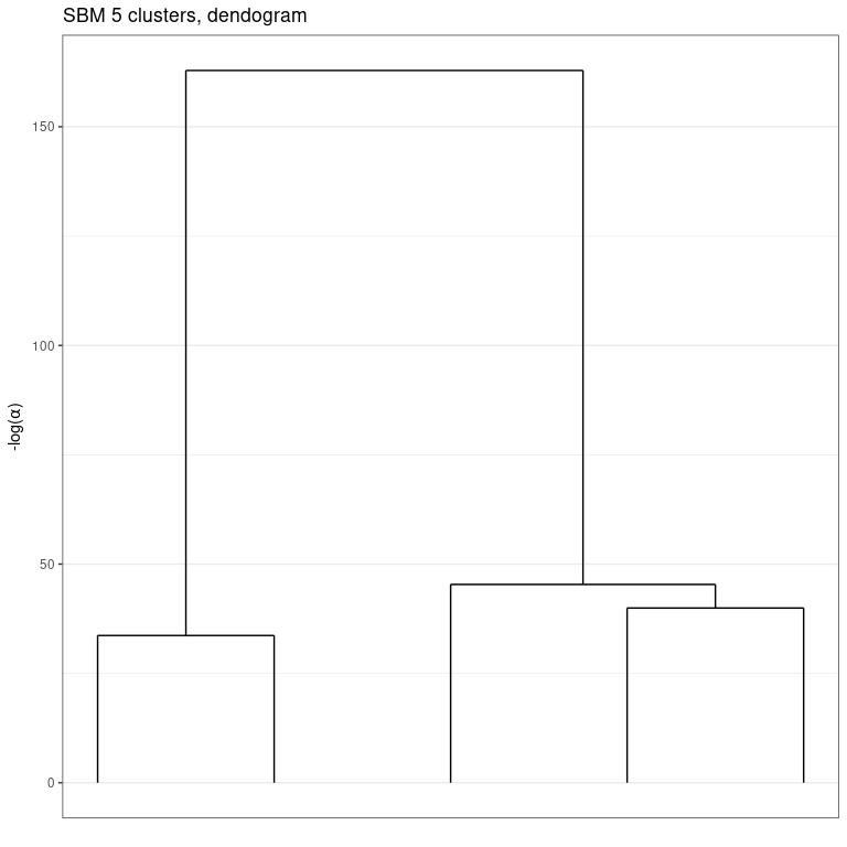
#> [5,] 0.000000000 0.000000000 0.043859649 0.427350427 0.73333333

Inspecting the hierarchy

An important aspect of the greed package is its hierarchical clustering algorithm which extract a set of nested partitions from K=K(sol) to K=1. This hierarchy may be visualized thanks to a dendogram representing the fusion order and the level of regularization − log (α) needed for each fusion.

plot(sol, type='tree') # try also: type="path"

Moreover, similar to standard hierarchical algorithm such as hclust, the cut() method allows you to extract a partition at any stage of the hierarchy. Its results is still an S4 object, and the S4 methods introduced earlier may again be used to investigate the results.

sol_K3 = cut(sol, K=3)
K(sol_K3)
#> [1] 3
table(Books$label,clustering(sol_K3)) %>% knitr::kable()

	1	2	3
c	1	6	42
l	38	5	0
n	2	8	3

Visualization

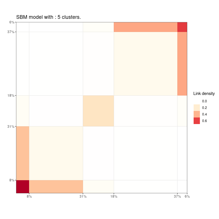
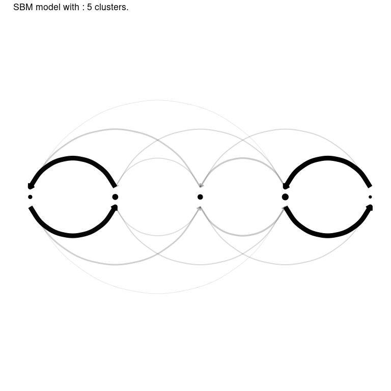
Finally, the greed package propose efficient and model-adapted visualization via the plot() methods. In this graph clustering example, the "blocks" and "nodelink" display the cluster-aggregated adjacency matrix and diagram of the graph respectively. Note that the ordering of the clusters is the same than the one computed for the dendrogram, greatly enhancing visualization of the hierarchical structure.

plot(sol,type='blocks')
plot(sol, type='nodelink')

Other models

As explained above, the greed package implements many standard models and the list may be displayed with

available_models()

Many plotting functions are available and, depending of the specified model, different type argument may be specified. For further information we refer to the vignettes linked above for each use case.

Using parallel computing

For large datasets, it is possible to use parallelism to speed-up the computations thanks to the future package. You only need to specify the type of back-end you want to use, before calling the ?greed function:

library(future)
plan(multisession, workers=2) # may be increased