This repository contains code for the paper Wave-Based Non-Line-of-Sight Imaging using Fast f-k Migration by David B. Lindell, Gordon Wetzstein, and Matthew O'Toole. The captured datasets can be downloaded separately from our project webpage.
 |
 |
|---|
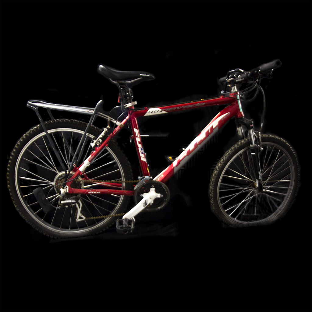
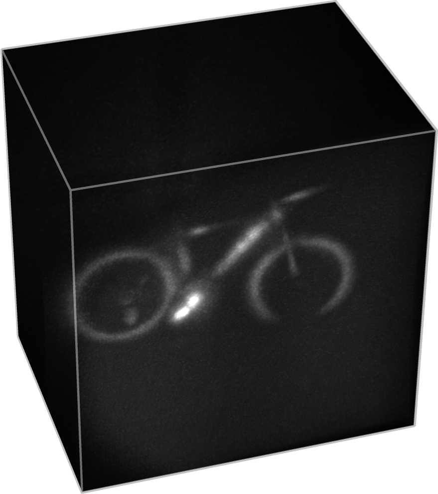
- Description: A white stone statue captured at approximately 1 m distance from the wall.
- Resolution: 512 x 512
- Scanned Area: 2 m x 2 m planar wall
- Integration times: 10 min., 30 min., 60 min., 180 min.
 |
 |
|---|
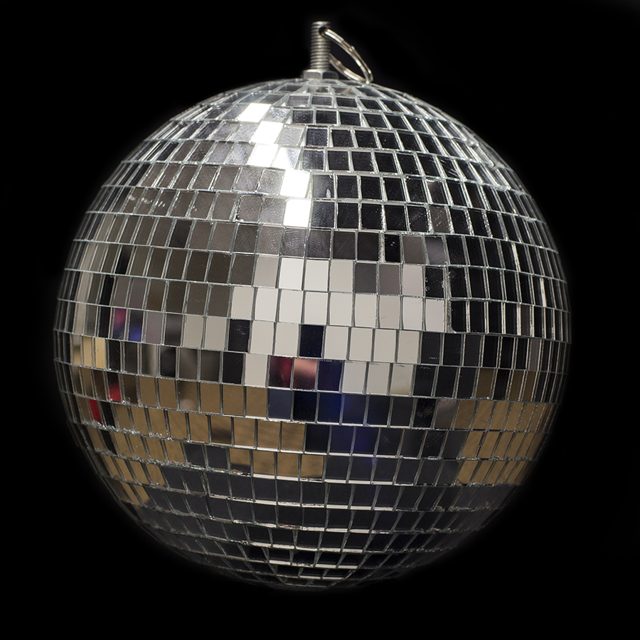
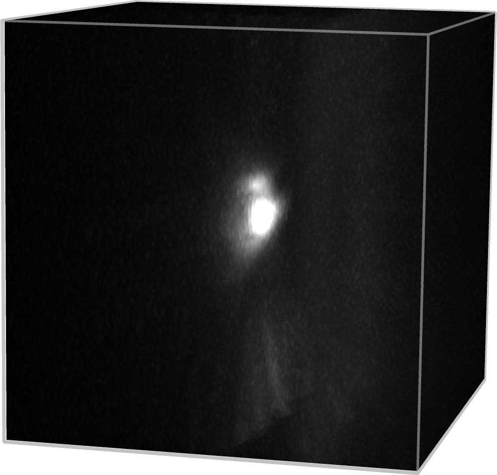
- Description: A specular disoball captured at approximately 1 m distance from the wall.
- Resolution: 512 x 512
- Scanned Area: 2 m x 2 m planar wall
- Integration times: 10 min., 30 min., 60 min., 180 min.
 |
 |
|---|
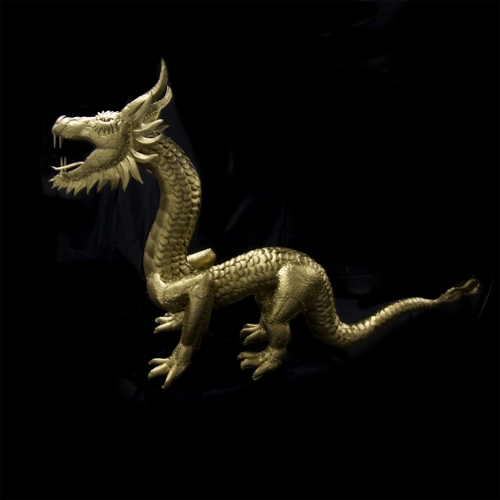
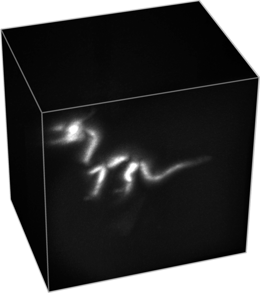
- Description: A glossy dragon captured at approximately 1 m distance from the wall.
- Resolution: 512 x 512
- Scanned Area: 2 m x 2 m planar wall
- Integration times: 15 sec., 1 min., 2 min., 10 min., 30 min., 60 min., 180 min.
 |
 |
|---|
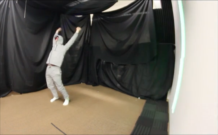
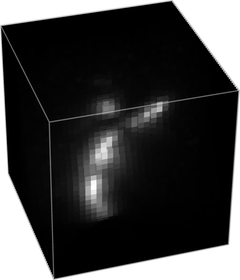
- Description: Two video captures of a person moving around in a retroreflective outfit.
- Resolution: 32 x 32 (4 fps), 64 x 64 (2 fps)
- Scanned Area: 2 m x 2 m planar wall
 |
 |
 |
|---|
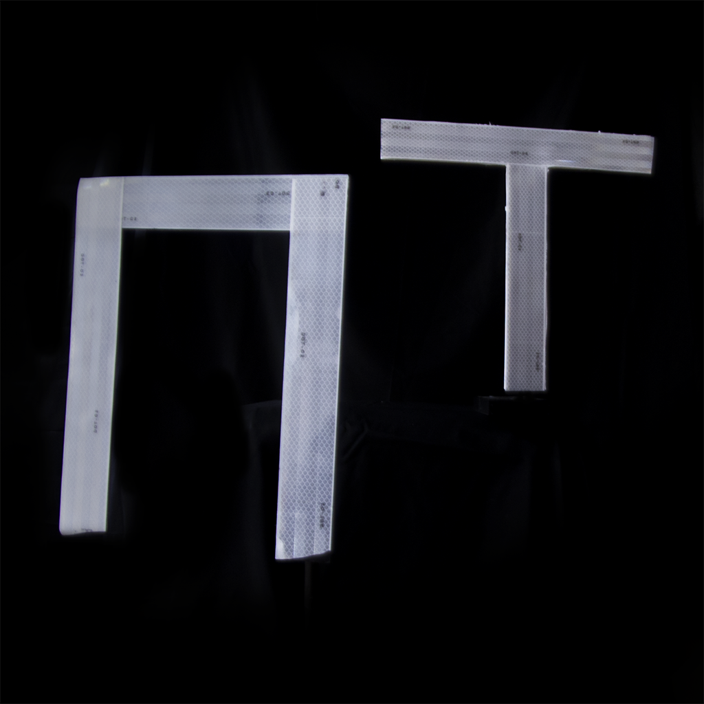
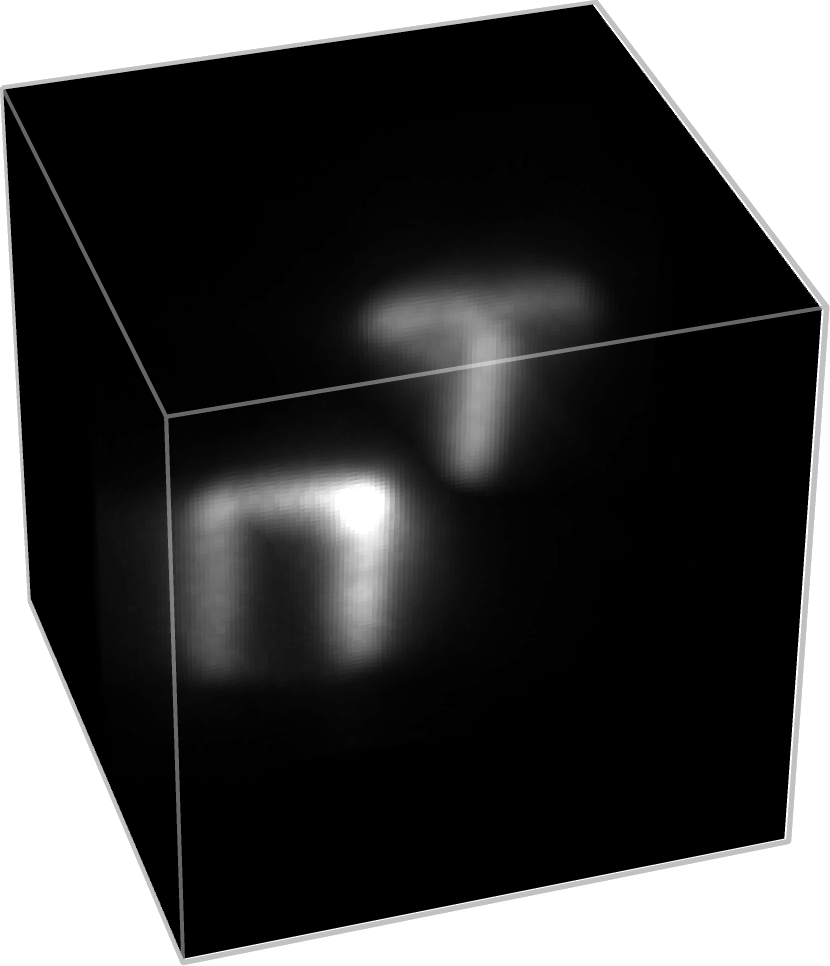
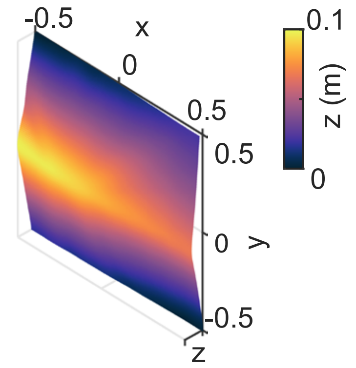
- Description: Two retroreflective letters captured at approximately 1 m distance from the wall by scanning a non-planar surface.
- Resolution: 128 x 128
- Scanned Area: 1 m x 1 m non-planar surface.
- Integration times: 150 sec.
 |
 |
 |
 |
|---|
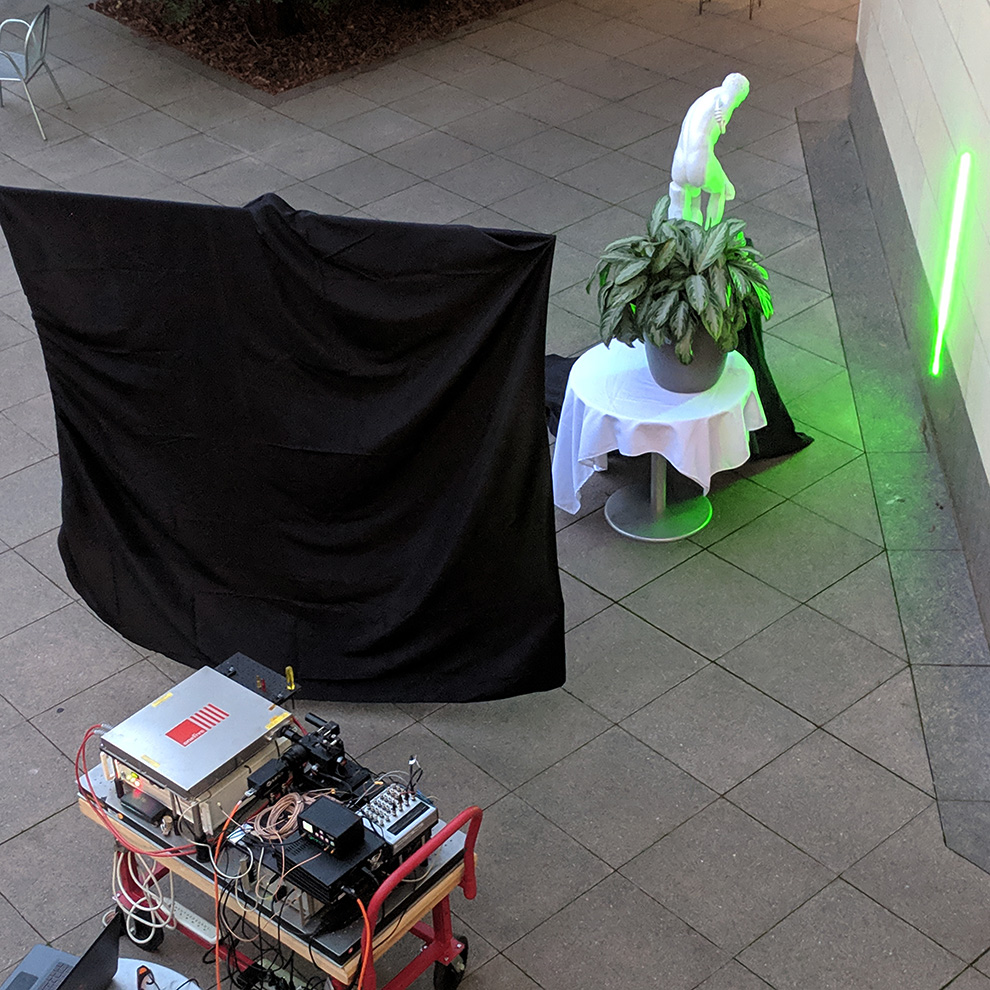
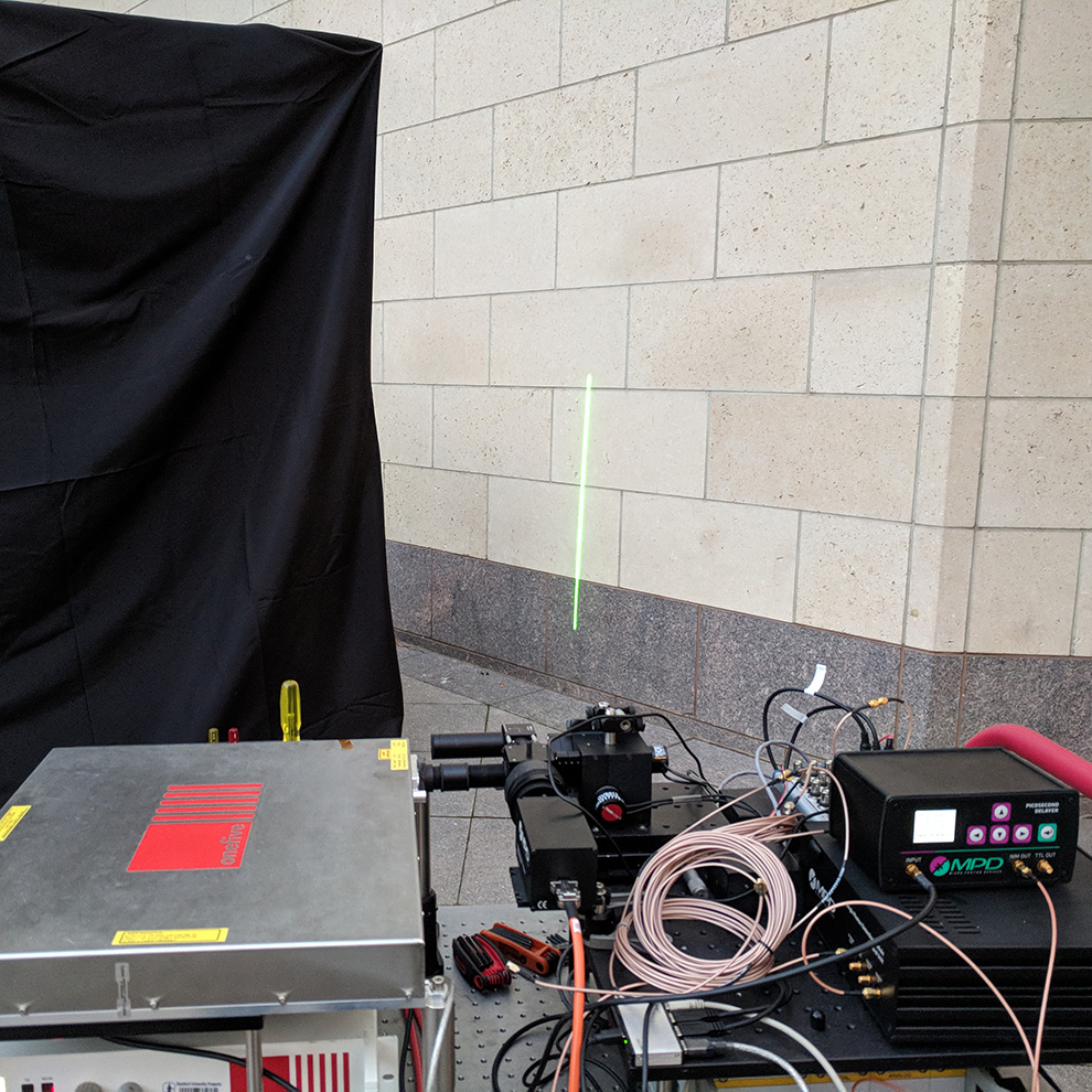
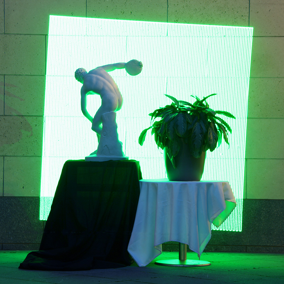
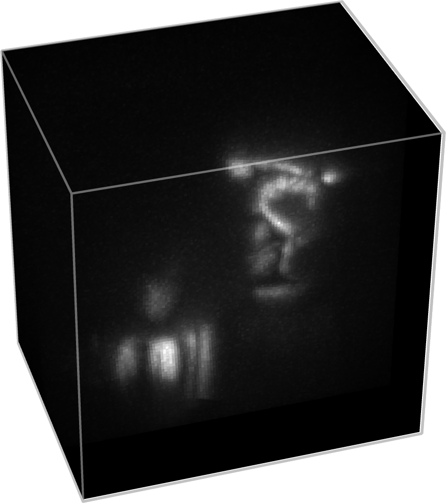
- Description: An outdoor scene captured by scanning the exterior of a building.
- Resolution: 128 x 128
- Scanned Area: 2 m x 2 m stone wall
- Integration times: 10 min., 30 min., 50 min.
 |
 |
|---|
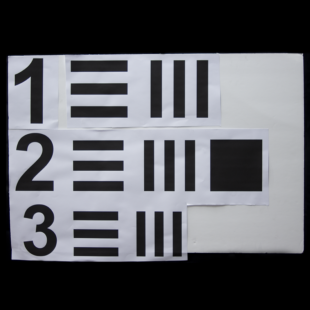
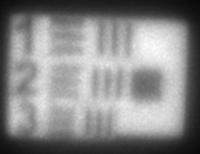
- Description: A resolution chart captured at approximately 1 m distance from the wall.
- Resolution: 512 x 512
- Scanned Area: 2 m x 2 m planar wall
- Integration times: 10 min., 30 min., 60 min., 180 min.
 |
 |
|---|
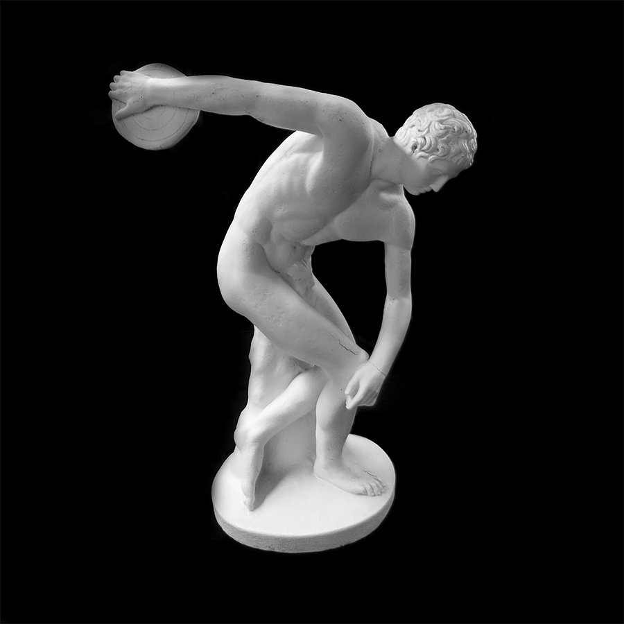
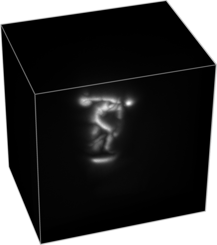
- Description: A white stone statue captured at approximately 1 m distance from the wall.
- Resolution: 512 x 512
- Scanned Area: 2 m x 2 m planar wall
- Integration times: 10 min., 30 min., 60 min., 180 min.
 |
 |
 |
|---|
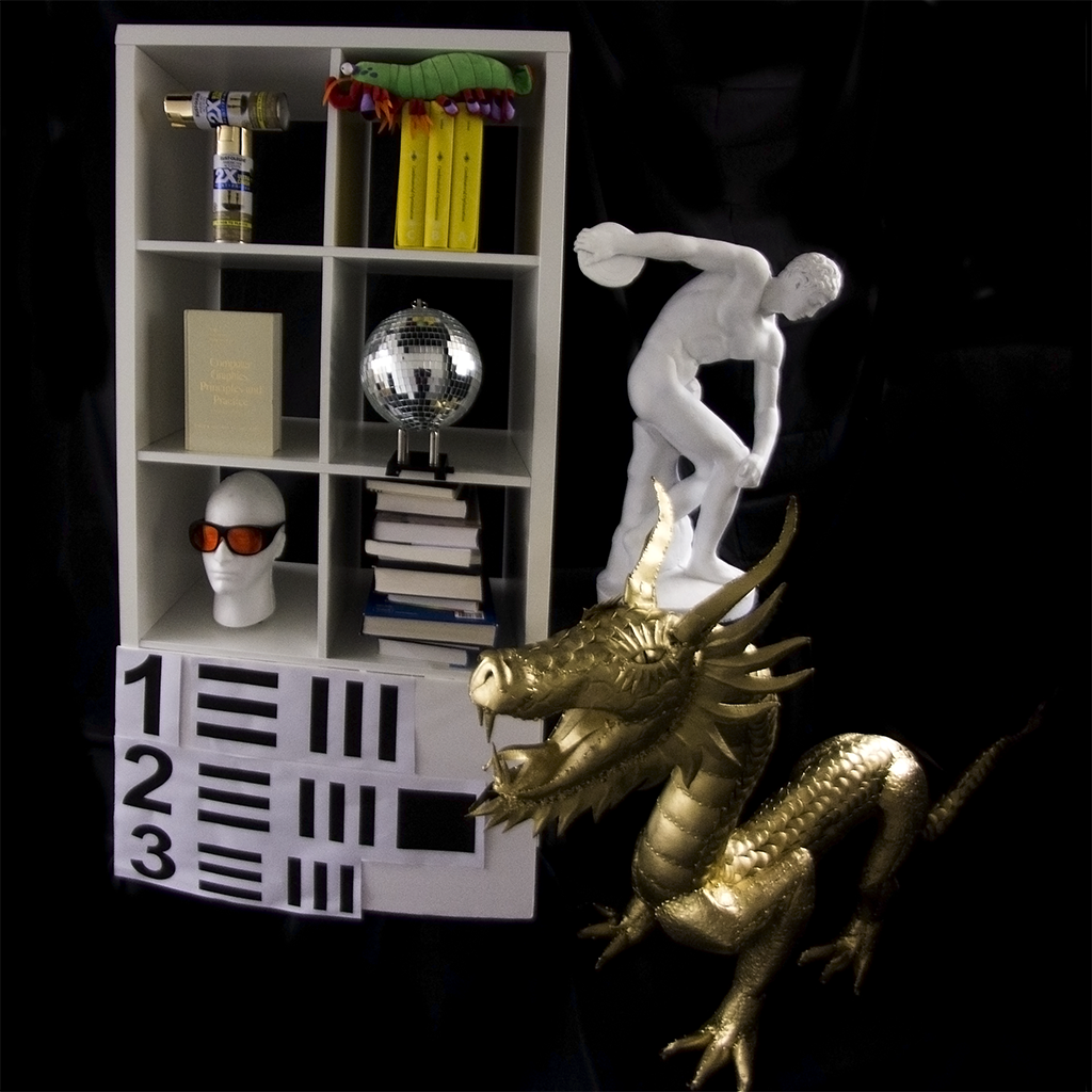
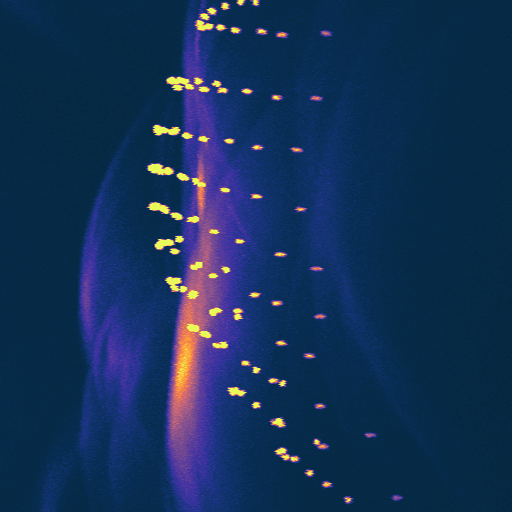
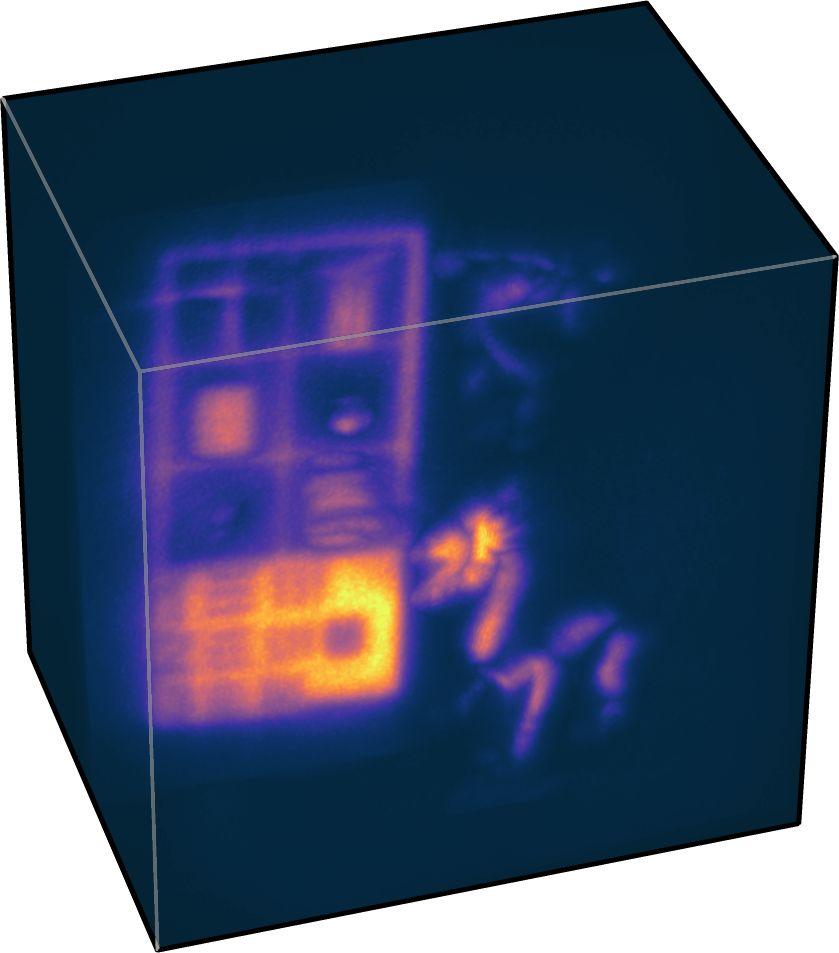
- Description: The teaser scene used in the paper which includes a number of objects, including a bookshelf, statue, dragon, and discoball.
- Resolution: 512 x 512
- Scanned Area: 2 m x 2 m planar wall
- Integration times: 10 min., 30 min., 60 min., 180 min.
The code/dataset should be organized as in the following directory tree
./dataset
	bike/
	discoball/
	dragon/
	interactive/
	nonplanar/
	outdoor/
	phase_retrieval/
	resolution/
	scenes/
	statue/
	teaser/
	util/
	cnlos_reconstruction.m
	demo.m
	hio_reconstruction.m
	LICENSE
    nonconfocal_reconstruction.m
	nonplanar_reconstruction.m
	README.md
Each of the folders contains a calibration file, measurement files, and example reconstructions.
The calibration files are named tof.mat and contain an image variable named tofgrid. This variable gives the time of flight in picoseconds to each scan point. Our example processing algorithms use this information to 'rectify' the measurements such that time zero coincides with the moment the light reflects off of the wall for all scan points. For the non-planar scan scenes we also include a variable, pos, which contains the 3D coordinate of each scan point relative to the confocal scanning hardware, and a tof_raw.mat file, which contains the raw time-of-flight measurement volume.
The measurement files are named meas_[10,30,60,180]min.mat, where the file name indicates the length of the exposure time in minutes. During the acquisition, we produce a complete scan every fifteen seconds, and so variable-length exposures can be compiled by accumulating the measurements over multiple scans. The files contain a 3D variable named meas of dimension 512x512x2048, with time being the last dimension. The time resolution of the measurements is 32 ps.
Note that our acquisition procedure involves using a gated sensor to prevent recording the overwhelmingly bright direct reflection from the wall. The time at which the gate turns on varies with distance to the scan surface and is visible in the measurements as a transition to non-zero photon counts. Latency in changing the gate delay results in a small subset of the measurements being gated out (set to zero) at the beginning of the scan period.
Finally, we include example reconstructions (at 512x512 spatial resolution) for the planar scenes using filtered backprojection (FBP) the Light-Cone Transform (LCT) and f-k migration methods. The corresponding files contain the reconstructed albedo volumes for each exposure time; the reconstruction method and exposure time are indicated by the filename.
These scenes were captured by rapidly scanning the wall at 2 or 4 fps and capturing 32 x 32 or 64 x64 spatial samples. The measurements capture a person moving around in a retroreflective outfit. The directory contains a set of 4D datafiles with 3D measurement volumes and f-k migration reconstructions for each captured frame. Videos of the scene captured with a conventional camera are also included.
The non-confocal processing is shown for an example scene from the Zaragosa NLOS dataset. Before running the function, download the non-confocal dataset from the Zaragosa webpage or using this direct link. We also provide example code for the NLOS dataset of Klein et al.. For convenience, we provide a direct download link to the example dataset we work with in a .mat format.
A non-planar scene consisting of two retroreflective letters was captured by scanning a deformed projector screen. We include the measurements, calibration files, and reconstructed 3D volumes using f-k migration or filtered backprojection. The nonplanar_reconstruction.m file can be run to load the measurements and generate the reconstructions. See the file for additional details.
A hybrid-input output phase retrieval algorithm can be used to process the teaser scene by running the hio_reconstruction.m file. We include the measurement volume used for processing, as well as full-resolution reconstructions of the initial volume and after 50 iterations of the algorithm.
Run the demo.m script to reconstruct a sample scene with FBP, LCT, f-k migration, and the phasor fields method by Liu et al. We also demonstrate how to reconstruct the interactive results, the non-planar scene, and how to run the phase retrieval algorithm.
License
The code and dataset are licensed under the following license:
Copyright (c) 2018, Stanford University
All rights reserved.
Redistribution and use in source and binary forms for academic and other non-commercial purposes with or without modification, are permitted provided that the following conditions are met:
Redistributions of source code, including modified source code, must retain the above copyright notice, this list of conditions and the following disclaimer.
Redistributions in binary form or a modified form of the source code must reproduce the above copyright notice, this list of conditions and the following disclaimer in the documentation and/or other materials provided with the distribution.
Neither the name of The Leland Stanford Junior University, any of its trademarks, the names of its employees, nor contributors to the source code may be used to endorse or promote products derived from this software without specific prior written permission.
Where a modified version of the source code is redistributed publicly in source or binary forms, the modified source code must be published in a freely accessible manner, or otherwise redistributed at no charge to anyone requesting a copy of the modified source code, subject to the same terms as this agreement.
THIS SOFTWARE IS PROVIDED BY THE TRUSTEES OF THE LELAND STANFORD JUNIOR UNIVERSITY "AS IS" AND ANY EXPRESS OR IMPLIED WARRANTIES, INCLUDING, BUT NOT LIMITED TO, THE IMPLIED WARRANTIES OF MERCHANTABILITY AND FITNESS FOR A PARTICULAR PURPOSE ARE DISCLAIMED. IN NO EVENT SHALL THE LELAND STANFORD JUNIOR UNIVERSITY OR ITS TRUSTEES BE LIABLE FOR ANY DIRECT, INDIRECT, INCIDENTAL, SPECIAL, EXEMPLARY, OR CONSEQUENTIAL DAMAGES (INCLUDING, BUT NOT LIMITED TO, PROCUREMENT OF SUBSTITUTE GOODS OR SERVICES; LOSS OF USE, DATA, OR PROFITS; OR BUSINESS INTERRUPTION) HOWEVER CAUSED AND ON ANY THEORY OF LIABILITY, WHETHER IN CONTRACT, STRICT LIABILITY, OR TORT (INCLUDING NEGLIGENCE OR OTHERWISE) ARISING IN ANY WAY OUT OF THE USE OF THIS SOFTWARE, EVEN IF ADVISED OF THE POSSIBILITY OF SUCH DAMAGE.
Contact
Questions can be addressed to David Lindell
Clone the git repo, download the datasets from our project webpage, and run demo.m in Matlab.