Mapper

This package provides a set of tools written in R/Rcpp for computing the mapper construction, and other related algorithms. Mapper was originally introduced in the article

Singh, Gurjeet, Facundo Mémoli, and Gunnar E. Carlsson. "Topological methods for the analysis of high dimensional data sets and 3d object recognition." SPBG. 2007.

Installation

The current development version can be installed with the devtools package:

require("devtools")
devtools::install_github("peekxc/Mapper")

A stable CRAN release is planned for the future.

Notes on installing

For some reason, R CMD check installs all packages listed in the Suggests field of the DESCRIPTION file. These must be installed, sometimes from source, without error across all platforms to make this package suitable for CRAN. This package includes multiple examples in either vignettes or example code that use large libraries like e.g. nloptr, geigen, rgl, etc. whose purpose is more illustrative than necessary for the package to function. As a result, the packages listed in Suggests are kept to a minimum to use the Mapper package functionally. Please refer to the documentation of individual functions for that functions dependencies.

Updates to simplextree

The mapper construction culminates in the nerve of a pullback cover, which is an abstract object called a simplicial complex. Mapper relies on the simplextree package to store, manipulate, and visualize simplicial complexes. While simplextree has been revamped, the current stable version of Mapper, and several development branches, depend on this older version; see this issue for details. In order to install and use Mapper, first install simplextree as follows:

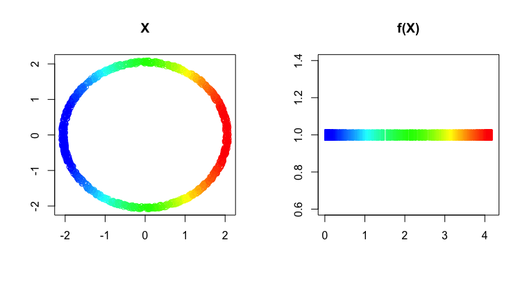
remotes::install_github("peekxc/simplextree", ref = "6e34926")

Usage

Given a data set, the first step to Mapper is to define a filter function. Here is an example using the noisy points sampled from the perimeter of a circle, similar to the example given by Example 3.2 in the original paper.

## Load package + the circle data set 
library("Mapper")
data("noisy_circle", package = "Mapper")

## Define filter values equal to the distance from each point to the left-most point in the circle 
left_pt <- noisy_circle[which.min(noisy_circle[, 1]),]
f_x <- matrix(apply(noisy_circle, 1, function(pt) (pt - left_pt)[1]))

Visualize the data and the results of the map

layout(matrix(1:2, nrow=1))
plot(noisy_circle, col = bin_color(f_x), main = "X", xlab = "", ylab = "")
plot(cbind(f_x, 1L), pch = "|", col = bin_color(f_x), main = "f(X)", xlab = "", ylab = "")

You can construct a mapper with R6 method chaining

## Define the main via chaining R6 methods
m <- MapperRef$new(noisy_circle)$
  use_filter(filter = matrix(f_x))$
  use_cover(cover="fixed interval", number_intervals=5L, percent_overlap=20)$
  use_distance_measure(measure="euclidean")$
  construct_k_skeleton(k=1L)
print(m)

Mapper construction with (8, 8) (0, 1)-simplices
Fixed Interval Cover: (number intervals = [5], percent overlap = [20]%)

The mapper is stored in a simplex tree. To get a quick overview of what the complex looks like use

print(m$simplicial_complex)

Simplex Tree with (8, 8) (0, 1)-simplices

Or print out the full trie structure

m$simplicial_complex$print_tree()

0 (h = 1): .( 1 2 )
1 (h = 1): .( 3 )
2 (h = 1): .( 4 )
3 (h = 1): .( 6 )
4 (h = 1): .( 5 )
5 (h = 1): .( 7 )
6 (h = 1): .( 7 )
7 (h = 0):

You can export to your favorite graph-based representation.

## Export to graph
m$simplicial_complex$as_adjacency_matrix()
# ...or m$simplicial_complex$as_adjacency_list()
# ...or m$simplicial_complex$as_edge_list()
# ...or m$simplicial_complex$as_list() for higher-dimension complexes

The vertices of the mapper are stored as a simple list

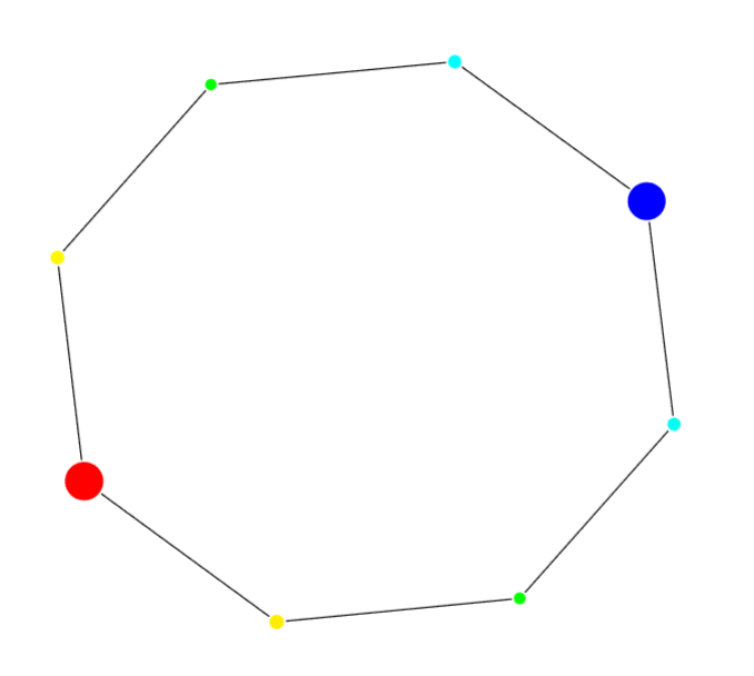
View(m$vertices)

To interact with the graph, consider using the pixiplex library.

library("pixiplex")
plot(m$as_pixiplex())

Additional Information