nowcaster is an R package for “nowcasting” epidemiological time series.
Every single system of notification has an intrinsic delay, nowcaster
can estimate how many counts of any epidemiological data of interest
(i.e., daily cases and death counts) by fitting a negative binomial
model to the time steps of delay between the onset date of the event,
(i.e., date of first symptoms for cases or date of occurrence of
death) and the date of report (i.e., date of notification of the case
or death).
nowcaster is based on the
R-INLA
and
INLA
packages for “Integrated Nested Laplace Approximation”
algorithm to Bayesian inference. INLA is a fast alternative to other
methods for Bayesian inference like MCMC. An introduction to INLA
can be found
here.
nowcaster is built for epidemiological emergency use, it was
constructed for the Brazilian Severe Acute Respiratory Illness (SARI)
surveillance database (SIVEP-Gripe).
To install nowcaster package simply run the code below in R:
if( !require(nowcaster, quietly = T) ){
  devtools::install_github("https://github.com/covid19br/nowcaster")
}
After installing you can load the typical library:
library(nowcaster)When the package is loaded it provides a LazyData file, sariBH, it is
an anonymized record of Severe Acute Respiratory Illness notified in the
city of Belo Horizonte, from March 2020 to April 2022. To load it
basically, write:
# Loading Belo Horizonte SARI dataset
data(sragBH)
And we take a look at the data:
head(sragBH)## # A tibble: 6 x 7
## DT_SIN_PRI DT_DIGITA CLASSI_FIN EVOLUCAO CO_MUN_RES Idade fx_etaria
## <date> <date> <dbl> <dbl> <dbl> <dbl> <fct>
## 1 2020-02-11 2020-03-05 4 1 310620 59 50 - 59
## 2 2020-01-21 2020-02-06 4 1 310620 79 70 - 79
## 3 2020-03-30 2020-04-17 4 1 310620 72 70 - 79
## 4 2020-03-26 2020-04-02 4 1 310620 82 80 +
## 5 2020-03-20 2020-04-13 4 1 310620 50 50 - 59
## 6 2020-04-07 2020-04-22 5 1 310620 74 70 - 79
It is a data.frame with 7 variables and 65,404 observations. We will make use of only the first two columns, “DT_SIN_PRI” (date of onset symptoms) and “DT_DIGITA” (recording date) as well as the column “Idade” (age in years) to make age-structured nowcasting.
Now we call the nowcasting function, it has by default the
parametrization to take the data and estimate it with non-structured data
form. The estimate fits a negative binomial distribution,
,
to the cases count at the time
with delay
,
is the dispersion parameter. The rate
is then parameterized in a log-linear format by a constant term added by
structured delay random effects and structured time random effects.
Hence, the model is given by the following:
where the intercept
follows is Gaussian distribution with a very large variance,
is follows a second-order random walk with precision
,
a first-order random walk with precision
.
The model is then completed by INLA default prior distributions for
,
,
and
.
See nbinom, rw1, and rw2 INLA help pages.
The call of the function is straightforward, it simply needs a dataset
as input, here the LazyData is loaded in the namespace of the package.
The function has 3 mandatory parameters, dataset for the parsing of
the dataset to be nowcasted, date_onset for parsing the column name
which is the date of onset of symptoms, and date_report which parses
the column name for the date of report of the cases. Here these columns
are “DT_SIN_PRI” and “DT_DIGITA”, respectively.
nowcasting_bh_no_age <- nowcasting_inla(dataset = sragBH,
                                        date_onset = DT_SIN_PRI,
                                        date_report = DT_DIGITA,
                                        data.by.week = T)
head(nowcasting_bh_no_age$total)
## # A tibble: 6 x 7
## Time dt_event Median LI LS LIb LSb
## <int> <date> <dbl> <dbl> <dbl> <dbl> <dbl>
## 1 17 2021-12-13 625 621 632 623 627
## 2 18 2021-12-20 695 687 709 692 699
## 3 19 2021-12-27 812 801 829 808 817
## 4 20 2022-01-03 886 871 906 880 893
## 5 21 2022-01-10 819 799. 847 811 826
## 6 22 2022-01-17 631 608 661 623 641
This calling will return only the nowcasting estimate and its Confidence
Interval (CI) for two different Credible intervals, LIb and LSb are
the max and min CI, respectively, with credibility of 50% and LI and
LS is the max and min CI, respectively, with a credibility of 95%.
nowcasting_inla has the option to return the curve when the
nowcasting estimate was set as the window of action of the model, if the
data.by.week parameter is flagged as TRUE it returns on the second
element of the output list the summarized data by week.
library(ggplot2)
library(dplyr)

dados_by_week <- nowcasting_bh_no_age$data |>
  filter(date_onset >= (Sys.Date()-270)) |>
  group_by(date_onset) |>
  summarise(n = n())

dados_by_week |>
  ggplot()+
  geom_line(data = dados_by_week, aes(date_onset, y = n, col = 'Observed'))+
  theme_bw()+
  theme(legend.position = "bottom", axis.text.x = element_text(angle = 90)) +
  scale_color_manual(values = c('grey50', 'black'), name = '')+
  scale_x_date(date_breaks = '2 weeks', date_labels = '%V/%y', name = 'Date in Weeks')+
  labs(x = '', y = 'Nº Cases')
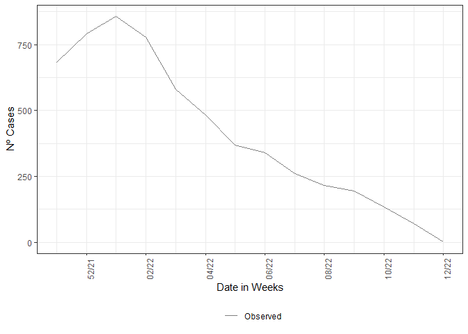
After this element is groped by and summarized by the onset of symptoms
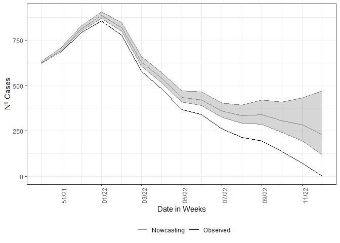
date, here DT_SIN_PRI, it is the epidemiological curve observed. For
example, how the estimate compares with the observed curve, we plot the
estimate and the epidemiological curve all together.
nowcasting_bh_no_age$total |>
  ggplot(aes(x = dt_event, y = Median, col = 'Nowcasting')) +
  geom_line(data = dados_by_week, aes(date_onset, y = n, col = 'Observed'))+
  geom_ribbon(aes(ymin = LI, ymax = LS, col = NA), alpha = 0.2, show.legend = F)+
  geom_line()+
  theme_bw()+
  theme(legend.position = "bottom", axis.text.x = element_text(angle = 90)) +
  scale_color_manual(values = c('grey50', 'black'), name = '')+
  scale_x_date(date_breaks = '2 weeks', date_labels = '%V/%y', name = 'Date in Weeks')+
  labs(x = '', y = 'Nº Cases')
This is an example where the estimate was done without considering any type of structure in data, which is the first assumption for the nowcasting.
Nowcasting a rising curve or a curve at any other moment can give quantitative support for decision-making, during the public health crises, the most needed is a way to anticipate, at least, what it is happening at the moment. Nowcasting is the tool for this type of questioning and can give insights on the data to support the needed decisions.
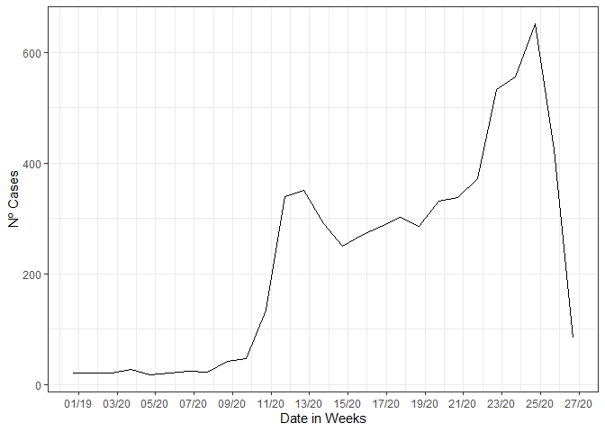
We start this section by cutting the original data at a moment of apparent decaying of the SARI hospitalization, for the city of Belo Horizonte, which had a prompt starting response to the COVID-19 pandemic. The pressure on the health system took more time than the rest of the country, and the data at the same time were showing a decay. We filter all cases entered until the 4th of July 2020 by the date of digitalization, a date that the cases show up in the database.
library(tidyverse)
library(lubridate)

## To see Nowcasting as if we were on the verge of rise in the curve
srag_now<-sragBH |>
  filter(DT_DIGITA <= "2020-07-04")

data_by_week<-data.w_no_age(dataset = srag_now,
                         date_onset = DT_SIN_PRI,
                         date_report = DT_DIGITA) |>
  group_by(date_onset) |>
  tally()

data_by_week |>
  ggplot(aes(x = date_onset,
             y = n))+
  geom_line()+
  theme_bw()+
  labs(x = 'Date of onset of symptons', y = 'Nº Cases')+
  scale_color_manual(values = c('grey50', 'black'), name = '')+
  scale_x_date(date_breaks = '2 weeks', date_labels = '%V/%y', name = 'Date in Weeks')
On this filtered data, we estimate the cases already that started its
date of onset of symptoms but were not yet reported, so there not in the
database. We just pass to the nowcasting_inla function, the dataset
filtered, flag for the columns where are the date_onset and
date_report, we add the flag for the function return the epidemic
curve by epiweek.
nowcasting_bh_no_age <- nowcasting_inla(dataset = srag_now,
                                        date_onset = DT_SIN_PRI,
                                        date_report = DT_DIGITA,
                                        data.by.week = T)
head(nowcasting_bh_no_age$data)
## # A tibble: 6 x 3
## date_report date_onset Delay
## <date> <date> <dbl>
## 1 2020-02-29 2020-02-08 3
## 2 2020-02-01 2020-01-18 2
## 3 2020-04-11 2020-03-28 2
## 4 2020-03-28 2020-03-21 1
## 5 2020-04-11 2020-03-14 4
## 6 2020-04-18 2020-04-04 2
Before we see the result of the nowcasting estimate we take a look on the intermediate part of the process of nowcasting, the delay triangle, which sets the objects for nowcasting. The delay triangle is only a a table where each unique amount of delay, (i.e. integer numbers of days or weeks) has passed between the date of onset and the date of report spread over each date of onset. The part that is closer to the present has less counts and has a lower amount of delay, this is trivial due to, the the system takes time to process the cases, the newer cases are lesser then the older ones, which already have time to be processed.
From the data in a weekly format, we mount the counts of cases by the amount of delay. By tabling the delay amount against the data of the onset of the first symptoms, we see the pattern of the delay for the cases.
data_triangle <- nowcasting_bh_no_age$data |>
  filter(Delay < 30) |>
  arrange(desc(Delay))
delay_triangle<-table(data_triangle$date_onset,
                      rev(data_triangle$Delay),
                      dnn = list("Date of Onset", "Delay"))
head(delay_triangle)
## Delay
## Date of Onset 0 1 2 3 4 5 6 7 8 9 10 11 12 13 14 15 16 17 18 19 20
## 2019-12-28 5 13 1 1 0 0 0 1 0 0 0 0 0 0 0 0 0 0 0 0 0
## 2020-01-04 3 15 1 0 0 1 0 0 0 0 0 0 0 0 0 0 0 0 0 0 0
## 2020-01-11 1 13 4 1 0 0 0 0 0 0 1 0 0 0 0 0 0 0 0 0 0
## 2020-01-18 5 17 3 0 0 0 0 0 0 0 1 0 0 0 1 0 0 0 0 0 0
## 2020-01-25 5 7 5 1 0 0 0 0 0 0 0 0 0 0 0 0 0 0 0 0 0
## 2020-02-01 3 12 3 1 0 0 0 0 0 0 0 1 0 0 0 0 0 0 0 0 0
We just look at the amount of cases with 30 weeks of delay or less, it
is the default maximum delay considered at nowcasting estimation. It can
be changed by the parameter Dmax.
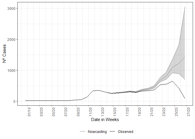
If this element is grouped by and summarized by the onset of symptoms
date, here DT_SIN_PRI, it is the epidemiological curve observed. For
example, we plot the estimate and the epidemiological curve all
together.
library(ggplot2)

dados_by_week <- nowcasting_bh_no_age$data %>%
  group_by(date_onset) %>%
  summarise(n = n())

nowcasting_bh_no_age$total |>
  ggplot(aes(x = dt_event, y = Median, col = 'Nowcasting')) +
  geom_line(data = dados_by_week, aes(date_onset, y = n, col = 'Observed'))+
  geom_ribbon(aes(ymin = LI, ymax = LS, col = NA), alpha = 0.2, show.legend = F)+
  geom_line()+
  theme_bw()+
  theme(legend.position = "bottom", axis.text.x = element_text(angle = 90)) +
  scale_color_manual(values = c('grey50', 'black'), name = '')+
  scale_x_date(date_breaks = '2 weeks', date_labels = '%V/%y', name = 'Date in Weeks')+
  labs(x = '', y = 'Nº Cases')
As expected, the nowcasting estimated a rise on a curve when it was observed a decaying. Adding to the plot what has happened in that period, with the data inserted posteriorly the period for when the nowcasting estimated the rising in the curve for SARI hospitalizations.
nowcasting_bh_no_age$total %>%
ggplot(aes(x = dt_event, y = Median, col = 'Nowcasting')) +
geom_line(data = dados_by_week, aes(date_onset, y = n, col = 'Observed'))+
geom_ribbon(aes(ymin = LI, ymax = LS, col = NA), alpha = 0.2, show.legend = F)+
geom_line()+
geom_line( data = sragBH %>%
filter(DT_SIN_PRI <= "2020-07-04") %>%
mutate(
D_SIN_PRI_2 = DT_SIN_PRI - as.numeric(format(DT_SIN_PRI, "%w"))
) %>%
group_by(D_SIN_PRI_2) %>%
tally(),
mapping = aes(x = D_SIN_PRI_2, y = n,
color = "Observed after one year")) +
theme_bw() +
theme(legend.position = "bottom", axis.text.x = element_text(angle = 90)) +
scale_color_manual(values = c('grey50', 'black', 'red'),
name = '')+
scale_x_date(date_breaks = '2 weeks', date_labels = '%V/%y', name = 'Date in Weeks')+
labs(x = '', y = 'Nº Cases')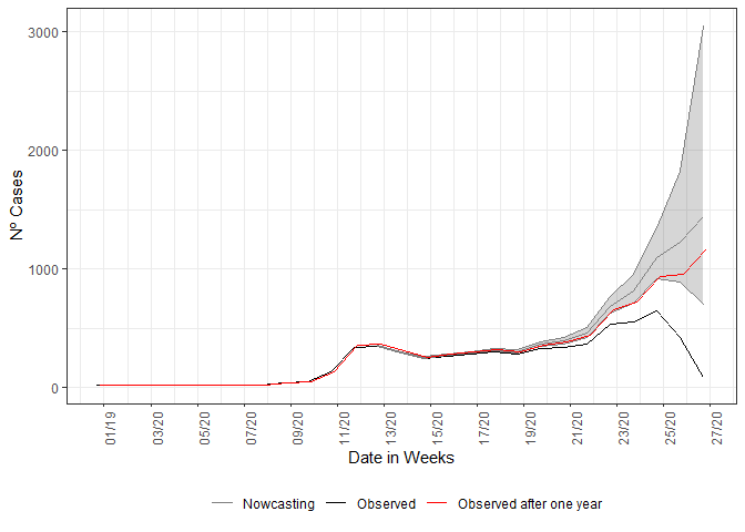 This ends the
first simple example when estimating the already started events but not
yet reported (i.e. nowcasting). The relevance of nowcasting for public
health decisions is given by the understanding that what is present in
the databases is only a picture of the real-time situation. The above
graph can help policymakers on what decisions to take in the face of a
rising curve of hospitalizations.
For the structured data the nowcasting_inla() fits again a Negative
binomial distribution to the cases count at the time
with delay
.
Differently, from the non-structured case, the model now gives random
effects on the delay distribution and and time distribution by each of
the age class chosen by the user to break the data. The model has the
form now:
where each age class,
,
has an intercept
following a Gaussian distribution with a very large variance, the
time-age random effects,
,
follow a joint multivariate Gaussian distribution with a separable
variance components an independent Gaussian term for the age classes
with precision
and a second-order random walk term for the time with precision
.
Analogously, the delay-age random effects,
,
follow a joint multivariate Gaussian distribution with a separable
variance components an independent Gaussian term for the age classes
with precision
and a first-order random walk term for the time with precision
.
The model is then completed by INLA default prior distributions for
,
,
,
and
.
See nbinom, iid, rw1, and rw2 INLA help pages.
This new model corrects the delay taking into account the effects of age
classes and the interactions of each age class between time and also
delay. Now the model needs a flag indicating which column on the
dataset will be used to break the data into age classes and how
the age classes will be split. This is given by the parameters age_col
and bins_age. We pass three additional parameters, data.by.week to
return the epidemiological curve out of a window of action of the nowcasting
estimate and return.age to inform we desire a nowcasting result in two
ways, the total aggregation estimate and the age-stratified estimate.
The calling of the function has the following form:
nowcasting_bh_age <- nowcasting_inla(dataset = sragBH,
                                     bins_age = "10 years",
                                     data.by.week = T,
                                     date_onset = DT_SIN_PRI,
                                     date_report = DT_DIGITA,
                                     age_col = Idade)
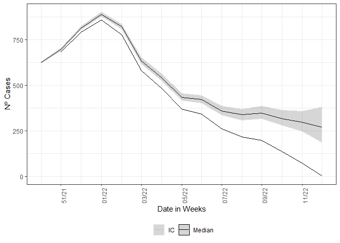
Each of the estimates returned by nowcasting_inla has the same form as
in the non-structured case. On the nowcasting estimates, it returns a
data.frame with the posterior median and 50% and 95% credible intervals,
(LIb and LSb) and (LI and LS) respectively.
library(ggplot2)

dados_by_week <- nowcasting_bh_age$data |>
  filter(date_onset >= (Sys.Date()-270)) |>
  group_by(date_onset) |>
  summarise(n = n())


nowcasting_bh_age$total |>
  ggplot(aes(x = dt_event, y = Median, col = 'Median'))+
  geom_line()+
  geom_line(data = dados_by_week, aes(date_onset, y = n))+
  geom_ribbon(aes(ymin = LI, ymax = LS, col = 'IC'), alpha = 0.2)+
  theme_bw()+
  theme(legend.position = "bottom", axis.text.x = element_text(angle = 90))+
  scale_color_manual(values = c('grey90', 'black'), name = '')+
  scale_x_date(date_breaks = '2 weeks', date_labels = '%V/%y', name = 'Date in Weeks')+
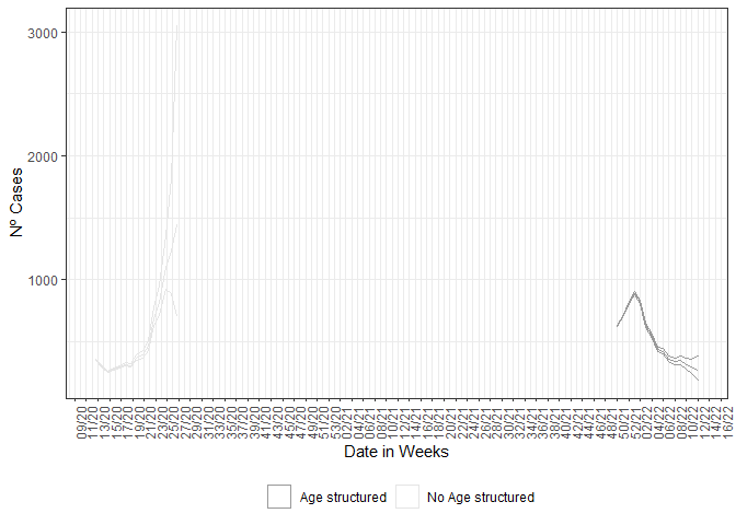
labs(x = '', y = 'Nº Cases')We can compare the estimates by each of the strategies, we plot the two estimates together:
nowcasting_bh_no_age$total$type <- "No Age structured"
nowcasting_bh_age$total$type <- "Age structured"


nowcasting_bh_total <- nowcasting_bh_age$total |>
  full_join(nowcasting_bh_no_age$total)

nowcasting_bh_total |>
  ggplot(aes(x = dt_event, y = Median, col = type))+
  geom_line(show.legend = F)+
  geom_ribbon(aes(ymin = LI, ymax = LS, fill = NULL), alpha = 0,
              show.legend = T)+
  theme_bw()+
  theme(legend.position = "bottom", axis.text.x = element_text(angle = 90))+
  scale_color_manual(values = c('grey60', 'grey90'), name = '')+
  scale_fill_manual(values = c('grey60', 'grey90'), name = '')+
  scale_x_date(date_breaks = '2 weeks', date_labels = '%V/%y', name = 'Date in Weeks')+
  labs(x = '', y = 'Nº Cases')
The estimates give different CIs, this is due to a better fitting when considering random effects by age class for the delays at time, this has to do with the different capabilities to respond at different ages. This is an empirical finding of this model.
sessionInfo()## R version 4.1.2 (2021-11-01)
## Platform: x86_64-w64-mingw32/x64 (64-bit)
## Running under: Windows 10 x64 (build 19042)
##
## Matrix products: default
##
## locale:
## [1] LC_COLLATE=Portuguese_Brazil.1252 LC_CTYPE=Portuguese_Brazil.1252
## [3] LC_MONETARY=Portuguese_Brazil.1252 LC_NUMERIC=C
## [5] LC_TIME=Portuguese_Brazil.1252
##
## attached base packages:
## [1] stats graphics grDevices utils datasets methods base
##
## other attached packages:
## [1] lubridate_1.8.0 forcats_0.5.1 stringr_1.4.0 purrr_0.3.4
## [5] readr_2.1.2 tidyr_1.2.1 tibble_3.1.8 tidyverse_1.3.2
## [9] dplyr_1.0.10 ggplot2_3.3.6 nowcaster_0.2.2 badger_0.2.1
##
## loaded via a namespace (and not attached):
## [1] httr_1.4.3 jsonlite_1.7.3 splines_4.1.2
## [4] tmvnsim_1.0-2 modelr_0.1.8 sn_2.0.1
## [7] assertthat_0.2.1 BiocManager_1.30.18 rvcheck_0.2.1
## [10] sp_1.5-0 highr_0.9 stats4_4.1.2
## [13] yulab.utils_0.0.5 googlesheets4_1.0.0 cellranger_1.1.0
## [16] yaml_2.2.2 numDeriv_2016.8-1.1 pillar_1.8.1
## [19] backports_1.4.1 lattice_0.20-45 glue_1.6.1
## [22] digest_0.6.29 RColorBrewer_1.1-3 rvest_1.0.2
## [25] colorspace_2.0-3 htmltools_0.5.2 Matrix_1.3-4
## [28] pkgconfig_2.0.3 broom_1.0.0 haven_2.4.3
## [31] scales_1.2.1 tzdb_0.2.0 MatrixModels_0.5-0
## [34] googledrive_2.0.0 generics_0.1.3 farver_2.1.1
## [37] ellipsis_0.3.2 withr_2.5.0 cli_3.1.1
## [40] mnormt_2.0.2 crayon_1.5.1 readxl_1.3.1
## [43] magrittr_2.0.2 evaluate_0.15 fs_1.5.2
## [46] fansi_1.0.3 xml2_1.3.3 tools_4.1.2
## [49] hms_1.1.1 gargle_1.2.0 lifecycle_1.0.2
## [52] reprex_2.0.1 munsell_0.5.0 compiler_4.1.2
## [55] rlang_1.0.5 grid_4.1.2 rstudioapi_0.13
## [58] INLA_21.11.22 labeling_0.4.2 rmarkdown_2.13
## [61] gtable_0.3.0 DBI_1.1.2 R6_2.5.1
## [64] knitr_1.39 fastmap_1.1.0 utf8_1.2.2
## [67] rprojroot_2.0.3 dlstats_0.1.5 desc_1.4.1
## [70] stringi_1.7.6 Rcpp_1.0.7 parallel_4.1.2
## [73] vctrs_0.4.1 dbplyr_2.1.1 tidyselect_1.1.2
## [76] xfun_0.29


-blue.svg)

