
The repository has been modified from Amantur Amatov and is an unofficial PyTorch implementation of the 2022 paper Music Source Separation with Band-split RNN (BSRNN) with some additional modifications to compete in the Sound Demixing Challenge (2023) - "Label Noise" Track. Huge thank you to both for developing and promoting this work!
- Problem Statement
- Background
- Datasets
- Exploratory Data Analysis (EDA)
- Architecture
- Conclusions
- Dependencies
- Inference
- Train your model
- Repository structure
- Citing
Audio source separation has been a topic of interest for quite some time, but has gained increasing attention recently due an increase in computing power and the capabilities of neural networks. Source separation can be implemented for a number of purposes, including speech clarity improvement, noise cancellation, or in our case separating individual instruments from a song. There are many use cases for this instrument separation technology, like music remixing, music information retrieval, and music education. This work seeks to review and improve upon current methods of audio source separation as well introduce robust training methods for circumstances when training data is "noisy" or not entirely clean.
When listening to music, humans inately can pick out the instruments within the complex mix of sounds. For example, it is trivial to pick out the drum set, guitar, bass, and of course the vocalist. However, there is no way to retrieve these isolated instruments that our mind "separates" or picks out from the music. It would follow that if our brains can process music in this manner, it is possible to develop algorithms that can do the same.
Methods of music source separation have been around in various forms for quite some time, but only recently has the ability to separate audio in high fidelity begun to be possible. This is due to the significant increase in computing capability over the recent years that has made training complex neural networks feasible. These "deep neural networks" (DNNs) can be trained on audio data by providing the fully "mixed" song as well as the isolated instrument "stem" to act as the target. The network then can learn how to pick out the frequencies and patterns that correlate to the individual instrument.
Since 2018, there have been many improvements on methods of source separation using neural networks. While many metrics can describe the performance of a model, it has become standard to use Signal-to-Distortion ratio (SDR) as the primary model performance metric. Below is a chart that demonstrates the improvement of various methods since 2018. Models were measured on how they performed on the MUSDB18 dataset.

Figure: Audio Source Separation Methods (source: paperswithcode.com)
| Rank | Model | SDR (avg) | SDR (vocals) | SDR (drums) | SDR (bass) | SDR (other) | Extra Training Data | Paper | Year |
|---|---|---|---|---|---|---|---|---|---|
| 1 | Sparse HT Demucs (fine tuned) | 9.2 | 9.37 | 10.83 | 10.47 | 6.41 | Y | Hybrid Transformers for Music Source Separation | 2022 |
| 2 | Hybrid Transformer Demucs (find tuned) | 9 | 9.2 | 10.08 | 9.78 | 6.42 | Y | Hybrid Transformers for Music Source Separation | 2022 |
| 3 | Band-Split RNN (semi-sup.) | 8.97 | 10.47 | 10.15 | 8.16 | 7.08 | Y | Music Source Separation with Band-split RNN | 2022 |
| 4 | Band-Split RNN | 8.24 | 10.01 | 9.01 | 7.22 | 6.7 | N | Music Source Separation with Band-split RNN | 2022 |
| 5 | Hybrid Demucs | 7.68 | 8.13 | 8.24 | 8.76 | 5.59 | N | Hybrid Spectrogram and Waveform Source Separation | 2021 |
| 6 | KUIELab-MDX-Net | 7.54 | 9 | 7.33 | 7.86 | 5.95 | N | KUIELab-MDX-Net: A Two-Stream Neural Network for Music Demixing | 2021 |
| 7 | CDE-HTCN | 6.89 | 7.37 | 7.33 | 7.92 | 4.92 | N | Hierarchic Temporal Convolutional Network With Cross-Domain Encoder for Music Source Separation | 2022 |
| 8 | Attentive-MultiResUNet | 6.81 | 8.57 | 7.63 | 5.88 | 5.14 | N | An Efficient Short-Time Discrete Cosine Transform and Attentive MultiResUNet Framework for Music Source Separation | 2022 |
| 9 | DEMUCS (extra) | 6.79 | 7.29 | 7.58 | 7.6 | 4.69 | Y | Music Source Separation in the Waveform Domain | 2019 |
| 10 | CWS-PResUNet | 6.77 | 8.92 | 6.38 | 5.93 | 5.84 | N | CWS-PResUNet: Music Source Separation with Channel-wise Subband Phase-aware ResUNet | 2021 |
| 11 | D3Net | 6.68 | 7.8 | 7.36 | 6.2 | 5.37 | Y | D3Net: Densely connected multidilated DenseNet for music source separation | 2020 |
| 12 | Conv-TasNet (extra) | 6.32 | 6.74 | 7.11 | 7 | Y | Conv-TasNet: Surpassing Ideal Time-Frequency Magnitude Masking for Speech Separation | 2018 | |
| 13 | UMXL | 6.316 | 7.213 | 7.148 | 6.015 | 4.889 | Y | Open-Unmix - A Reference Implementation for Music Source Separation | 2021 |
| 14 | DEMUCS | 6.28 | 6.84 | 6.86 | 7.01 | 4.42 | N | Music Source Separation in the Waveform Domain | 2019 |
| 15 | TAK2 | 6.04 | 7.16 | 6.81 | 5.4 | 4.8 | Y | MMDenseLSTM: An efficient combination of convolutional and recurrent neural networks for audio source separation | 2018 |
| 16 | D3Net | 6.01 | 7.24 | 7.01 | 5.25 | 4.53 | N | D3Net: Densely connected multidilated DenseNet for music source separation | 2021 |
| 17 | Spleeter (MWF) | 5.91 | 6.86 | 6.71 | 5.51 | 4.02 | Y | Spleeter: A Fast And State-of-the Art Music Source Separation Tool With Pre-trained Models | 2019 |
| 18 | LaSAFT+GPoCM | 5.88 | 7.33 | 5.68 | 5.63 | 4.87 | N | LaSAFT: Latent Source Attentive Frequency Transformation for Conditioned Source Separation | 2020 |
| 19 | X-UMX | 5.79 | 6.61 | 6.47 | 5.43 | 4.64 | N | All for One and One for All: Improving Music Separation by Bridging Networks | 2020 |
| 20 | Conv-TasNet | 5.73 | 6.81 | 6.08 | 5.66 | 4.37 | N | Conv-TasNet: Surpassing Ideal Time-Frequency Magnitude Masking for Speech Separation | 2018 |
| 21 | Sams-Net | 5.65 | 6.61 | 6.63 | 5.25 | 4.09 | N | Sams-Net: A Sliced Attention-based Neural Network for Music Source Separation | 2019 |
| 22 | Meta-TasNet | 5.52 | 6.4 | 5.91 | 5.58 | 4.19 | N | Meta-learning Extractors for Music Source Separation | 2020 |
| 23 | UMX | 5.33 | 6.32 | 5.73 | 5.23 | 4.02 | N | Open-Unmix - A Reference Implementation for Music Source Separation | 2019 |
| 24 | Wavenet | 3.5 | 3.46 | 4.6 | 2.49 | 0.54 | N | End-to-end music source separation: is it possible in the waveform domain? | 2018 |
| 25 | STL2 | 3.23 | 3.25 | 4.22 | 3.21 | 2.25 | N | Wave-U-Net: A Multi-Scale Neural Network for End-to-End Audio Source Separation | 2018 |
The raw audio dataset all of these models were tested on is the MUSDB18 dataset. Each song is organized into "vocals", "drums", "bass", and "other" stem files and "mixture" fully mixed track.
For the "Label Noise" MDX track, a separate private dataset was provided that had been artificially manipulated to simulate "un-clean" data. For example, a track that may be labeled "bass" could actually be a recording of drums. Or a vocal track may "accidentally" have the hi hat and guitar mixed in. The manipulation was random and varied so that manual processing of these tracks was not feasible. This was done in order to promote the development of a model and training method robust to noisy data.
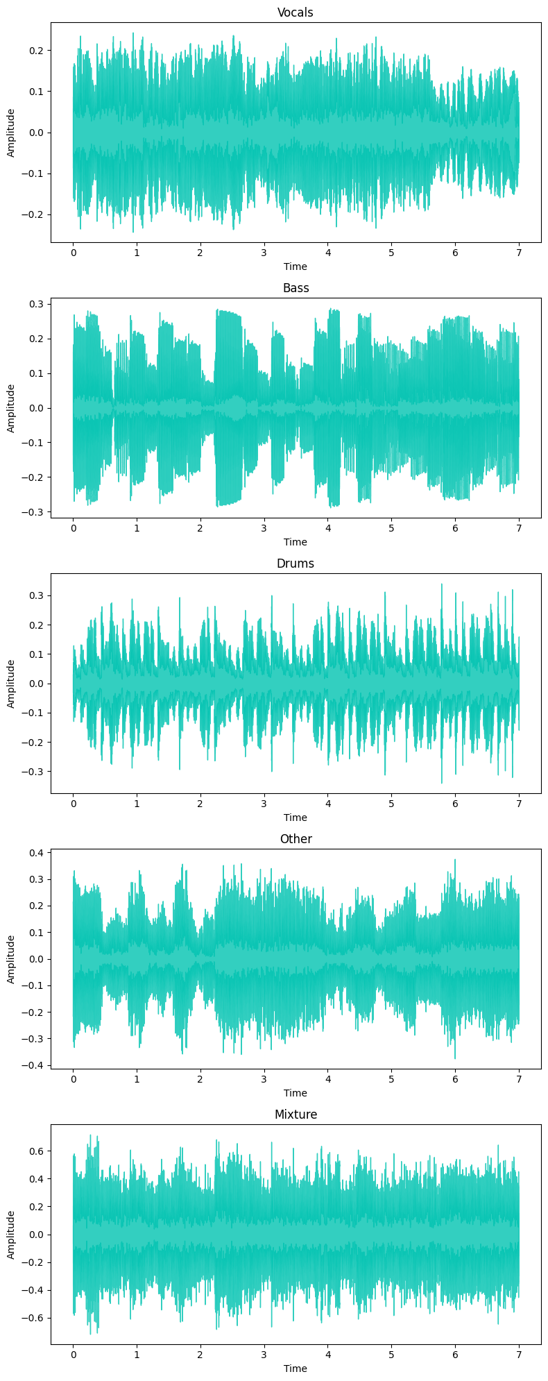
- The waveform of the data shows the oscillations of pressure amplitude over time. This is effectively a "raw" format of audio data.
- It is defined by the sampling frequency and bit depth.
- The sampling frequency refers to how many samples of audio are played back per second (i.e. 44.1kHz means that every second, 44,100 samples are played). This determines the upper bound of frequencies that can be represented by the audio signal.
- The bit depth refers to how precise the amplitude values are determining the dynamic range of an audio signal (i.e. 16-bit depth can represent 65,536 unique numbers, resulting in approx. 96dB of dynamic range)
- To simplify, the sampling rate essentially controls the resolution of the x-axis and the bit depth controls the resolution of the y-axis
- While it can often be hard to glean information by visually inspecting waveforms, you can see different characteristics in each different instrument's waveform.
- Vocals - Notice how the vocals have a more consistently full signal (likely holding notes until the dropoff in the last second).
- Bass - Notice how the bass appears to almost have "blocks" of waves at similar amplitudes (likely holding a singl note).
- Drums - Notice how the drums have many spikes in amplitude (potentially snare or bass drum hits).
- Other - Less can be gleaned from other, as it likely contains a mixture of other instruments. However, there does seem to be some amplitude fluctations that somewhat consistent to the bas signal.
- Mixture - Notice how the mixture is the fullest signal with the highest amplitude. Because all signals have been summed together, it is incredibly challenging to glean anything from this signal from visual inspection.
- For further analysis, the signals need to be brought into the frequency domain.
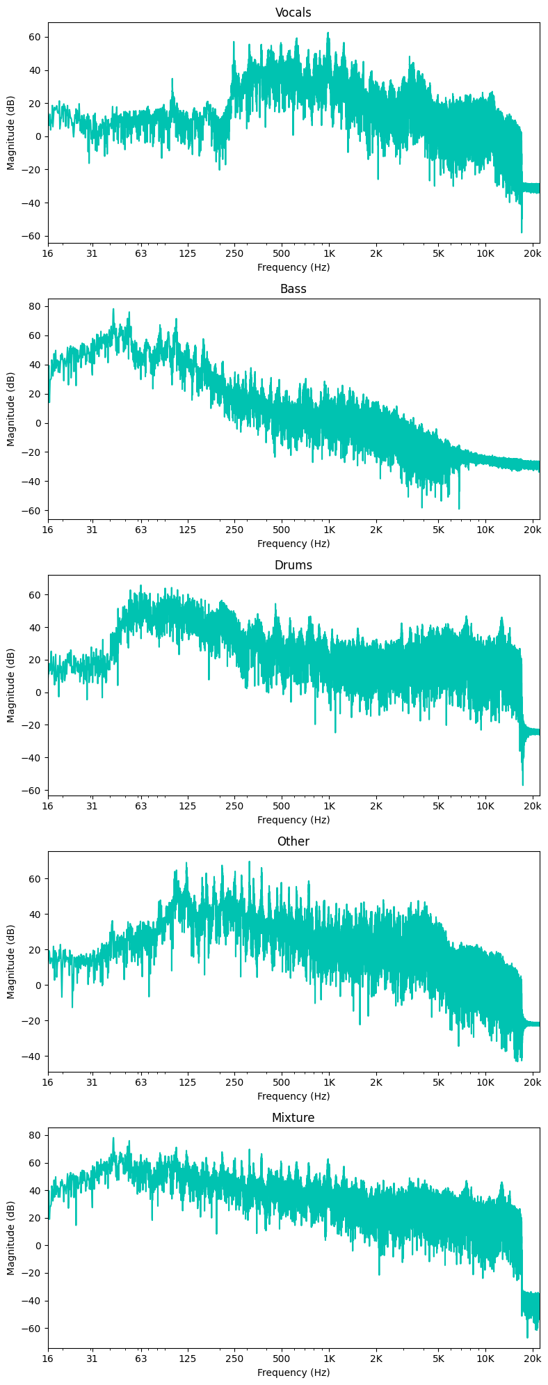
- The spectrum of a waveform shows the magnitude (in dB) of the signal per frequency.
- Notice there is no time component here, rather the magnitude (dB) is with reference to frequencies of the entire audio signal (in this case 30 sec clip)
- While the plot below shows the spectrum for the entire signal, we will be using this concept to take the spectrum of small pieces of the signal to reintroduce a time component when we create spectrograms next.
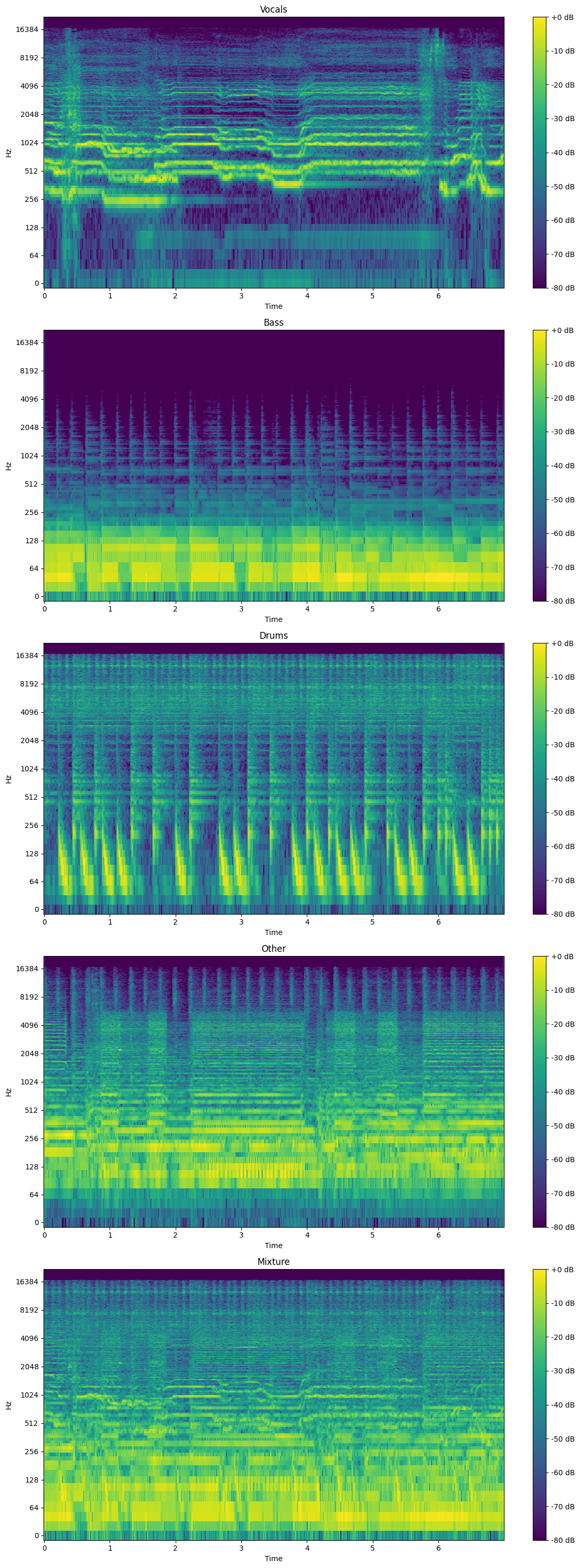
- A spectrogram is the combination of a waveform and spectrum plot, resulting in frequency magnitude (in dB) over time.
- It has been scaled so that 0 dB is the maximum value.
- Notice how patterns emerge in the light-green and yellow, looking like diagonal lines that move up and down. These patterns correspond to specific attributes of the music, such as melodies.
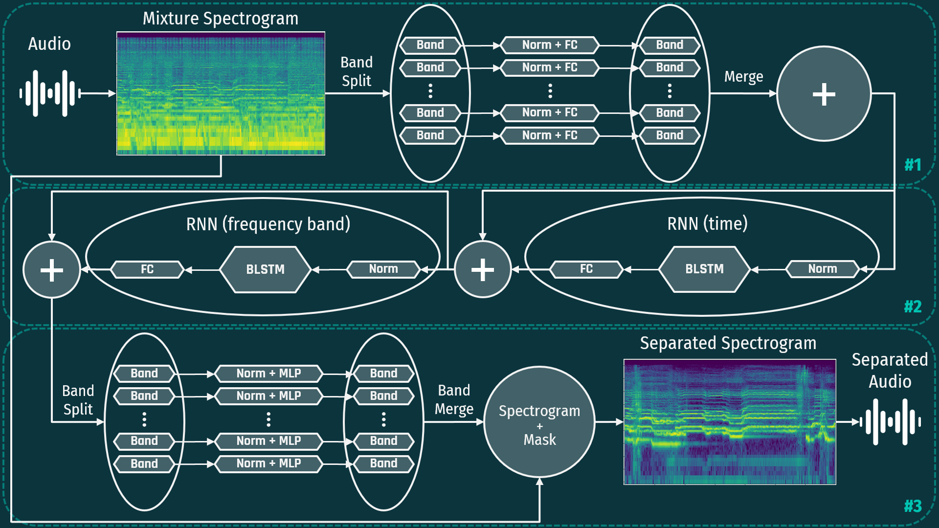
This section details the architecture of the entire system. The model framework consists of 3 modules:
- Band-split module
- Band and sequence separation modeling module
- Mask estimation module
Being that it is a fairly complex structure, each module will be described in detail in order to create a total understanding of the BSRNN framework.
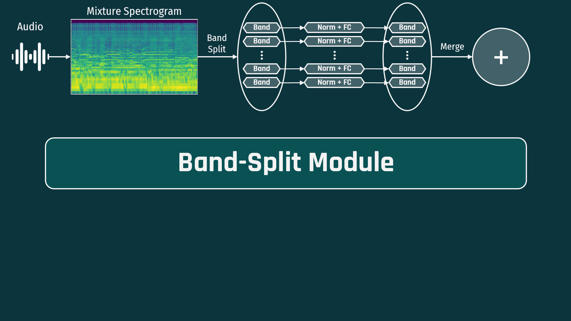
In the first module, audio is converted to a spectrogram by the short-time Fourier transform (STFT). The spectrogram is then split into sub-bands. The number of sub-bands and their bandwidth can be adjusted to bias the system separately for each target instrument. Sub-bands are then normalized and sent through one fully-connected dense layer per band. Dense layers are then merged to be sent through the next module
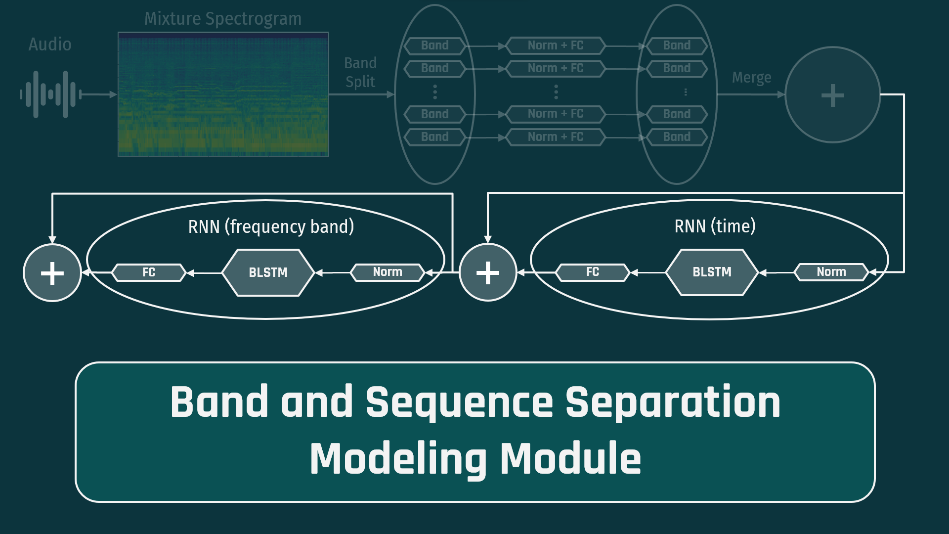
In the second module, the data is fed through a pair of RNNs, which consists of normalization, a bi-directional LSTM (long short term memory network) and the a fully connected layer. The first RNN is fed with the data across the time dimension and the second is fed with the data across the frequency band dimension. This pair of RNNs can be repeated multiple times to improve the complexity that the network can learn. For example, this implementation used 12 layers per the paper specifications. The data is then combined and moves on to the final module.
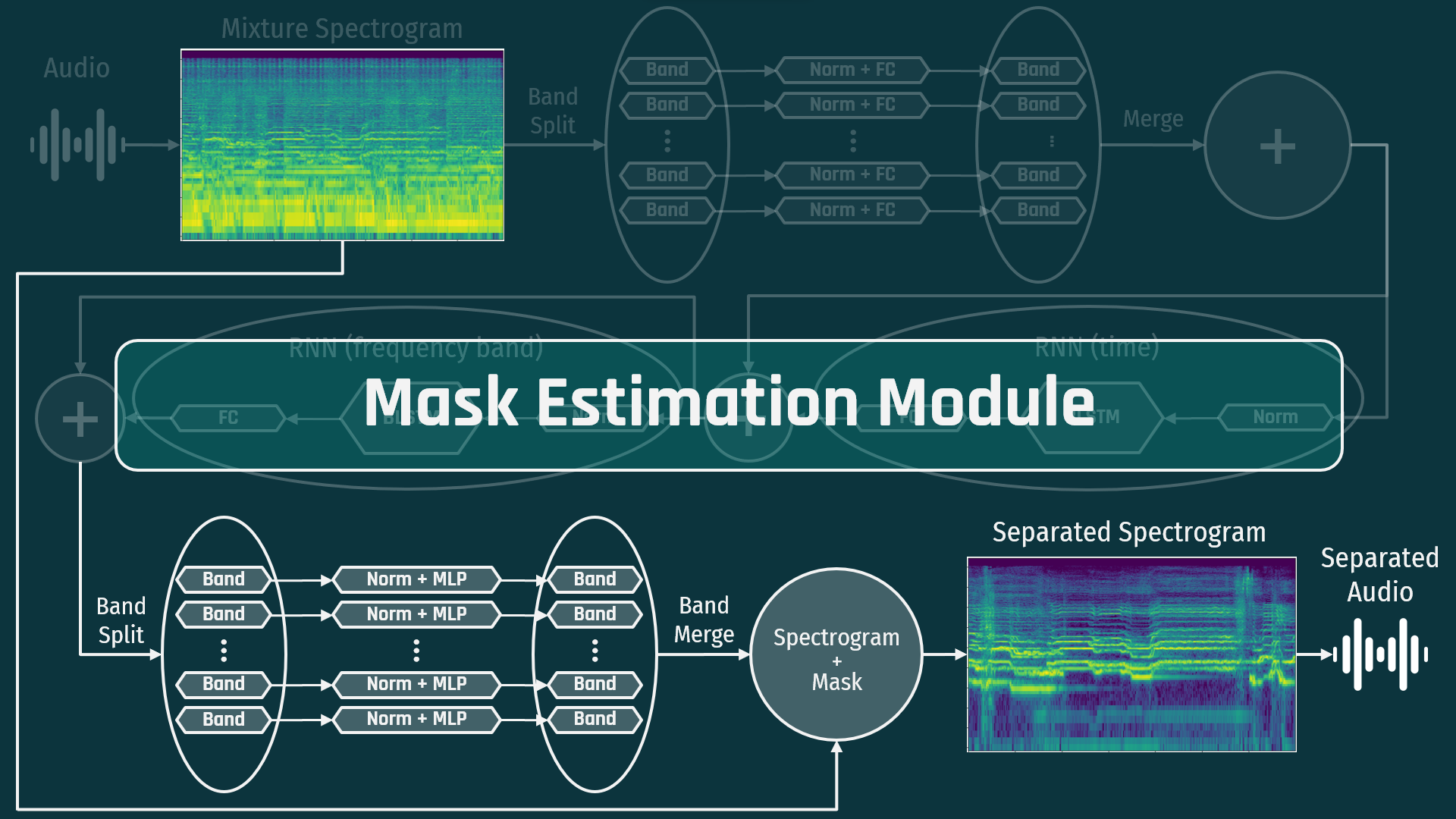
In the final module, the data is band-split again, normalized, and sent through an multi-layer perceptron (MLP - 1 in, 1 hidden, 1 out) per band with the hyperbolic tangent activation function. This produces a spectrogram “mask” that is then multiplied by the original signal to generate the target spectrogram. This is then compared to the training data and the loss is calculated and backpropagated through the network to update all weights.
This Band-Split RNN framework offers high performance with both optimized training data as well as “noisy” training data. This is because the model can be biased with knowledge about characteristics of instruments. This is a recently published novel framework and still has a great deal of possible tuning, particularly regarding instruments other than vocals.
Some of the reasons for reduction in performance for the MDX-23 Label Noise competition include:
- Limited resources (single GPU)
- Limited implementation and training time
- Not enough preprocessing & cleaning of training data
- No hyperparameter tuning
- The 4 sources of Vocals, Bass, Drums, and Other are not all-encompassing.
- Create datasets that consist of more diverse stems (e.g. acoustic guitar, strings, etc.)
- Better choice of band-splitting (currently determined through rough grid-search)
- Improved pre-processing pipeline
- E.g. Use another model to classify instruments and filter appropriately to clean training data
- Tune hyperparameters:
- Frame size (how much audio is analysis at a time: Used 3 seconds
- Hop size (spacing between frames, aka overlap): 2.5 seconds
- Adjust dimensions in Band Split and Mask Estimation modules
- Adjust dimensions and number of BLSTM layers in Band and Sequence module
Python version - 3.10.
To install dependencies, run:
pip install -r requirements.txt
Additionally, ffmpeg should be installed in the venv.
If using ``conda[example_vocals.mp3](..%2F..%2F..%2FDownloads%2Fexample_vocals.mp3), you can run:
conda install -c conda-forge ffmpeg
All scripts should be run from src directory.
Train/evaluation/inference pipelines support GPU acceleration.
To activate it, specify the following env variable:
export CUDA_VISIBLE_DEVICES={DEVICE_NUM}
To run inference (demix) on audio file(s), firstly, you need to train your own model or download checkpoints.
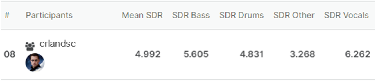
Current checkpoints were trained only on the "Label Noise" data from AIcrowd. These checkpoints were limited due to computing resources and time for the MDX competition. Further training would improve performance.
To improve results to match the BSRNN paper, the model must be trained on clean MUSDB18 data and additional fine-tuning data.
Available checkpoints (via Hugging Face):
| Target | Approx. Size | Epoch | SDR |
|---|---|---|---|
| Vocals | 500MB | 246 | 6.262 |
| Bass | 500MB | 296 | 5.605 |
| Drums | 500MB | 212 | 4.831 |
| Other | 500MB | 218 | 3.268 |
After you download the .pt or .ckpt file, put it into ./saved_models/{TARGET}/ directory.
Afterwards, run the following shell script:
python3 inference.py [-h] -i IN_PATH -o OUT_PATH [-t TARGET] [-c CKPT_PATH] [-d DEVICE]

options:
  -h, --help            show this help message and exit
  -i IN_PATH, --in-path IN_PATH
                        Path to the input directory/file with .wav/.mp3 extensions.
  -o OUT_PATH, --out-path OUT_PATH
                        Path to the output directory. Files will be saved in .wav format with sr=44100.
  -t TARGET, --target TARGET
                        Name of the target source to extract.
  -c CKPT_PATH, --ckpt-path CKPT_PATH
                        Path to model's checkpoint. If not specified, the .ckpt from SAVED_MODELS_DIR/{target} is used.
  -d DEVICE, --device DEVICE
                        Device name - either 'cuda', or 'cpu'.
You can customize inference via changing audio_params in ./saved_models/{TARGET}/hparams.yaml file. Here is vocals example:
python3 inference.py -i ../example/example.mp3 -o ../example/ -t vocals
There is still some work going on with training better checkpoints, and at this moment I've trained only (pretty bad) vocals extraction model.
In this section, the model training pipeline is described.
The paper authors used the MUSDB18-HQ dataset to train an initial source separation model.
You can access it via Zenodo.
This version of the model was trained on the "Label Noise" data from AIcrowd.
After downloading, set the path to this dataset as an environmental variable
(you'll need to specify it before running the train and evaluation pipelines):
export MUSDB_DIR={MUSDB_DIR}
To speed up the training process, instead of loading entire files, we can precompute the indices of fragments we need to extract. To select these indices, the proposed Source Activity Detection (SAD) algorithm was used.
To read the musdb18 dataset and extract salient fragments according to the target source, use the following script:
python3 prepare_dataset.py [-h] -i INPUT_DIR -o OUTPUT_DIR [--subset SUBSET] [--split SPLIT] [--sad_cfg SAD_CFG] [-t TARGET [TARGET ...]]

options:
  -h, --help            show this help message and exit
  -i INPUT_DIR, --input_dir INPUT_DIR
                        Path to directory with musdb18 dataset
  -o OUTPUT_DIR, --output_dir OUTPUT_DIR
                        Path to directory where output .txt file is saved
  --subset SUBSET       Train/test subset of the dataset to process
  --split SPLIT         Train/valid split of train dataset. Used if subset=train
  --sad_cfg SAD_CFG     Path to Source Activity Detection config file
  -t TARGET [TARGET ...], --target TARGET [TARGET ...]
                        Target source. SAD will save salient fragments of vocal audio.
Output is saved to {OUTPUT_DIR}/{TARGET}_{SUBSET}.txt file. The structure of the file is as follows:
{MUSDB18 TRACKNAME}\t{START_INDEX}\t{END_INDEX}\n
To train the model, a combination of PyTorch-Lightning and hydra was used.
All configuration files are stored in the src/conf directory in hydra-friendly format.
To start training a model with given configurations, just use the following script:
python train.py
To configure the training process, follow hydra instructions.
By default, the model is trained to extract vocals. To train a model to extract other sources, use the following scripts:
python train.py train_dataset.target=bass model=bandsplitrnnbass
python train.py train_dataset.target=drums model=bandsplitrnndrums
python train.py train_dataset.target=other
To load the model from a checkpoint, in the script include:
ckpt_path=path/to/checkpoint.ckpt
After training is started, the logging folder will be created for a particular experiment with the following path:
src/logs/bandsplitrnn/${now:%Y-%m-%d}_${now:%H-%M}/
This folder will have the following structure:
├── tb_logs
│   └── tensorboard_log_file    - main tensorboard log file
├── weights
│   └── *.ckpt                  - lightning model checkpoint files.
└── hydra
│   └──config.yaml              - hydra configuration and override files
└── train.log                   - logging file for train.py
To start evaluating a model with given configurations, use the following script:
python3 evaluate.py [-h] -d RUN_DIR [--device DEVICE]

options:
  -h, --help            show this help message and exit
  -d RUN_DIR, --run-dir RUN_DIR
                        Path to directory checkpoints, configs, etc
  --device DEVICE       Device name - either 'cuda', or 'cpu'.
This script creates test.log in the RUN_DIR directory and writes the uSDR and cSDR metrics there
for the test subset of the MUSDB18 dataset.
The structure of this repository is as following:
├── src
│   ├── conf                        - hydra configuration files
│   │   └── **/*.yaml
│   ├── data                        - directory with data processing modules
│   │   └── *.py
│   ├── files                       - output files from prepare_dataset.py script
│   │   └── *.txt
│   ├── model                       - directory with modules of the model
│   │   ├── modules
│   │   │   └── *.py
│   │   ├── __init__.py
│   │   ├── bandsplitrnn.py         - file with the model itself
│   │   └── pl_model.py             - file with Pytorch-Lightning Module for training and validation pipeline
│   ├── notebooks                   - directory with notebooks for audio pre-processing
│   │   └── *.py
│   ├── saved_models                - directory with model checkpoints and hyper-parameters for inference
│   │   ├── bass
│   │   │   ├── bass.ckpt
│   │   │   └── hparams.yaml
│   │   ├── drums
│   │   │   ├── drums.ckpt
│   │   │   └── hparams.yaml
│   │   ├── other
│   │   │   ├── other.ckpt
│   │   │   └── hparams.yaml
│   │   └── vocals
│   │       ├── vocals.ckpt
│   │       └── hparams.yaml
│   ├── utils                       - directory with utilities for evaluation and inference pipelines
│   │   └── *.py
│   ├── evaluate.py                 - script for evaluation pipeline
│   ├── inference.py                - script for inference pipeline
│   ├── prepare_dataset.py          - script for dataset preprocessing pipeline
│   ├── separator.py                - separator class, which is used in evaluation and inference pipelines
│   └── train.py                    - script for training pipeline
├── images
├── presentation
├── .gitignore
├── README.md
└── requirement.txt
To cite this paper, please use:
@misc{https://doi.org/10.48550/arxiv.2209.15174,
  doi = {10.48550/ARXIV.2209.15174},
  url = {https://arxiv.org/abs/2209.15174},
  author = {Luo, Yi and Yu, Jianwei},
  keywords = {Audio and Speech Processing (eess.AS), Machine Learning (cs.LG), Sound (cs.SD), Signal Processing (eess.SP), FOS: Electrical engineering, electronic engineering, information engineering, FOS: Electrical engineering, electronic engineering, information engineering, FOS: Computer and information sciences, FOS: Computer and information sciences},
  title = {Music Source Separation with Band-split RNN},
  publisher = {arXiv},
  year = {2022},
  copyright = {Creative Commons Attribution Non Commercial Share Alike 4.0 International}
}