Solving Linear Inverse Problems Using the Prior Implicit in a Denoiser

arXiv paper: https://arxiv.org/abs/2007.13640
Zahra Kadkhodaie, Eero P. Simoncelli

Contents of this repository:

1. Pre-trained denoisers

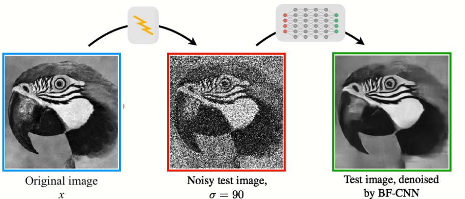
The denoisers directory contains several universal CNN denoisers, pre-trained for removing Gaussian noise from natural images with the objective of minimizing mean square error. All denoisers are "blind": they can remove noise of any standard deviation, and this standard deviation does not need to be specified. The implicit embedded prior depends on the architecture of the denoiser as well as the images in the training set. The denoisers directory contains a separate folder for each architecture, with code specified in code/network.py. Within each architecure directory, there are multiple folders containing variants of that denoiser trained on different datasets and noise ranges.

2. Code

The code directory contains the python code for the algorithm, the pre-trained denoisers, and helper functions.

3. Test_images

The test_images directory contains several commonly used color and grayscale image datasets.

4. Demo

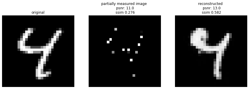
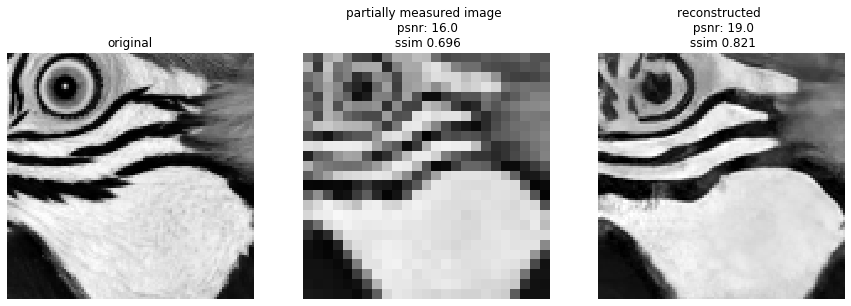
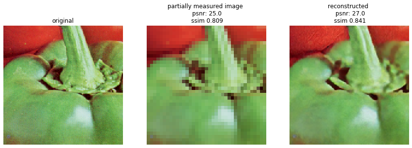
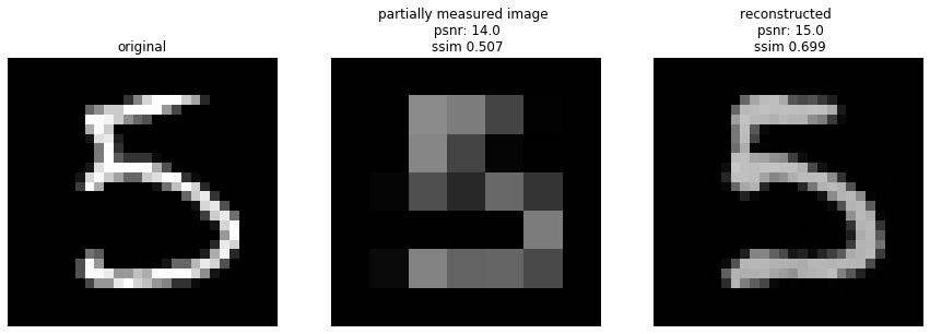
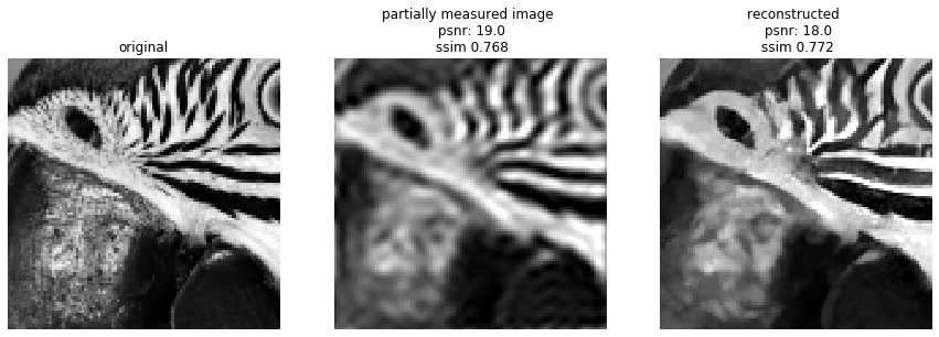
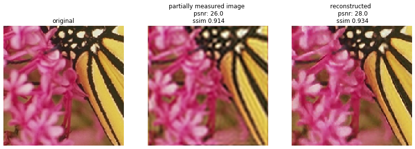
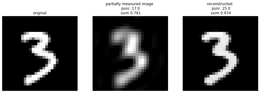
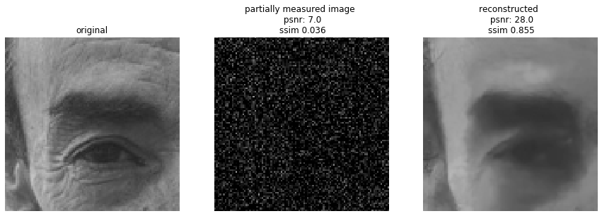
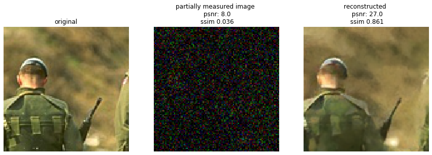
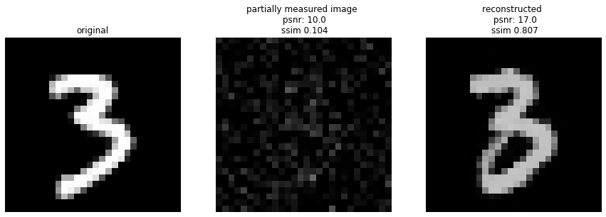
The notebook Demo.ipynb contains code for loading a pre-trained universal denoiser, and using it to draw samples from the image prior that is implicitly embedded within the denoiser (see paper). It also contains code for solving a set of linear inverse problems: inpainting, deblurring, super-resolution, randomly-dropped pixels, and compressive sensing. Notice that there is no additional training involved for solving these problems, and the same algorithm is used for all. The algorithm uses the prior embedded in the denoiser to generate the missing parts of the partially measured image.

Demo.ipynb can be executed on CPU or GPU computing platforms.

Requirements

You'll need python version 3.7.6 and the following packages to execute the code:

numpy 1.19.4
skimage 0.17.2
matplotlib 1.19.4
PyTorch 1.7.0
argparse 1.1
os
time
sys
gzip

Summary

Image priors, manifolds, and noisy observations

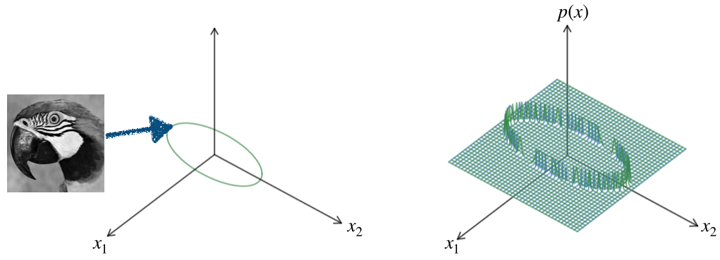
Visual images lie on a low-dimensional manifold, spanned by various natural deformations. Images on this manifold are approximately equally probable - at least locally. The probability of being a natural image, , is zero everywhere except for lying on the manifold.

An observed image, , contaminated with Gaussian noise, $z\sim \mathcal N(0,\sigma^2)$ is drawn from an observation density, , which is a Gaussian-blurred version of the image prior. Moreover, the family of observation densities over different noise variances, , forms a Gaussian scale-space representation of the prior, analogous to the temporal evolution of a diffusion process.

Least squares denoising

Given a noisy observation, , the least squares estimate of the true signal is the conditional mean of the posterior:

Exposing the implicit prior through Empirical Bayes estimation

For Gaussian noise contamination, Miyasawa (1961) showed that the least squares estimate can be written (exactly) as:

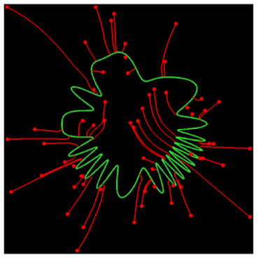
Unlike the standard formulation (an integral over the posterior density), this expresses the denoising operation in terms of the gradient of the prior predictive density, . For intuition, we show a two-dimensional simulation/visualization for a one-dimensional manifold (green curve), and three different noise amplititudes. End of red line segments shows the least-squares optimal denoising solution $\hat{x}$ for each noisy signal, :

Drawing samples from the implicit prior

Algorithm in a nutshell (see paper for details):

Use the denoiser-defined gradient to go uphill in probability
On each step, the effective noise decreases, and the effective prior becomes less blurred. The denoiser, and thus the gradient step size, automatically adapts to this.
This coarse-to-fine optimization procedure converges to a point on the manifold

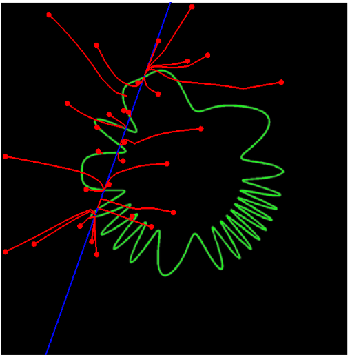
Below is a two-dimensional visualization of example trajectories of the sampling algorithm:

Click here to watch a video of the two-dimensional simulation.

When the method is used to sample an image, we can visualize points along these trajectories as sequences of images, . Below are three pairs of sequences, for the BF-CNN denoiser trained on (1) grayscale natural images (2) color natural images and (3) the MNIST dataset of handwritten digits. Each pair includes two sequences with different initial (leftmost) images, , and added noise, . Each sequence converges to a sample from the prior (manifold) implicit in the corresponding denoiser (rightmost images).

Solving linear inverse problems using the implicit prior

Given a set of linear measurements of an image, = , where M is a low-rank measurement matrix, we use an enhanced version of the algorithm to draw a sample of an image that satisfies these measurements (i.e., an image that lies at the intersection of the manifold and the hyperplane spanned by the column space of M). In the examples below, we show the simple (pseudo-inverse) image reconstructed from the measureents, as well as that obtained from our algorithm, for five different types of measurement matrices, M.

1. Inpainting

Here, the algorithm must fill in a missing block of pixels (i.e., the measurement consists of the pixels outside of the missing block). With different initializations and different additive noise, the algorithm arrives at different solutions (different points on the manifold). For each trained denoiser, we show three different samples, each of which looks natural.

2. Missing random pixels

The measurements consist of a randomly selected subset of 10% of the pixels.

3. Super-resolution

Measurements are averages of each (non-overlapping) block of 4x4 pixels.

4. Spectral super resolution

Measurements consist of 10% of Fourier coefficients (the lowest frequencies).

5. Random basis (compressive sensing)

Here, the measurement matrix contains random orthogonal unit vectors that span a subspace whose dimensionality is 10% of the dimensionality of the image. Thus, the measurements are the projections of the image onto a low-dimensional random subspace.

crystal-cheung/universal_inverse_problem