#Variational Autoencoders and Generative Adversarial Networks.
##Variational Autoencoder
Implemented in Tensorflow as defined at https://arxiv.org/pdf/1312.6114.pdf.
The variational autoencoder is a generative and probabilistic model that tries to create encodings that look as though they were sampled from a normal distribution.
This means that in order to generate a sample from the autoencoder we just need to generate a sample from a standard normal distribution, and run it through the decoder.
To construct and train the model we need to define a loss function as usual. However in variational inference we maximize the ELBO
ELBO = E[log p(x|z)] - DKL(q(z|x) || p(z))
The first term refers to maximizing the expected log likelihood. As we need the model to generate probabilities as outputs then we need to pass the logits of the decoder into a sigmoid function. Then, the expected log likelihood is calculated as follows.
xentropy = tf.nn.sigmoid_cross_entropy_with_logits(labels=X, logits=logits);
The second term refers to The KL Divergence between the normal distribution generated by the latent space and a standard normal distribution (although the codings are to limited to Gaussian distributions). It acts as a regularizer that forces to cluster, for example, digits with the same value but with different writings close in the euclidean space.
As tensorflow only provides the minimize function on each of its optimizers, then we have to minimize the -ELBO.
opt_step = tf.train.AdamOptimizer(learning_rate = self.learning_rate).minimize(-elbo)
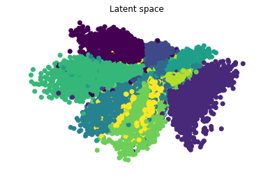
We can visualize the representations in the latent space of the training set and draw each cluster(digit) in a different color.
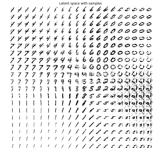
Another nice visualization is to verify the region in the latent space that will render a certain digit. We
do this by creating a grid in the latent space and reconstructing the digits that correspond to each point in
the grid.

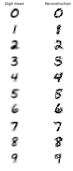
Finally we observe the differences between the mean presentation of each digit with its reconstruction using the posterior prediction.
A GAN is a neural network that is composed by a generator and a discriminator networks. The principal application of the GANs is to generate realistic images that can in turn be used in other supervised tasks.
The discriminator takes an image and its job is to decide whether it is real or fake. The generator produces fake images and tries to fool the discriminator by creating realistic images.
We can construct the discriminator as usual using convolutional, dropout and dense layers.
        conv1 = conv2d(X_in, filters = conv1_params[0], kernel_size = conv1_params[1], strides = conv1_params[2])
        conv1 = tf.layers.dropout(conv1, rate = dropout_rate)

        conv2 = conv2d(conv1, filters = conv2_params[0], kernel_size = conv2_params[1], strides = conv2_params[2])
        conv2 = tf.layers.dropout(conv2, rate = dropout_rate)

        conv3 = tf.layers.conv2d(conv2, filters = conv3_params[0], kernel_size = conv3_params[1], strides = conv3_params[2])
        conv3 = tf.layers.dropout(conv3, rate = dropout_rate)

        flatten = tf.layers.flatten(conv3);

        dense1 = dense(flatten, dense1_params[0])

        output = dense(dense1, dense2_params[0], activation = None)
For the generator we need to construct a special layer that behaves as the opposite of the convolutional layer. Generally, the output of the covolutional layer is a smaller image. Then the oppositive operation should output a larger image than the input.
We can't contruct a deconvolutional layer as actually the convolutional operational is destructive. However it suffices to look for an operation that spatially behaves the same: the output should be larger than the input. This layer in tensorflow is conv2d_transpose.
The remaining elements that are needed for the generator are dense and dropout layers.
        dense1 = dense(z, pp1[0]*pp1[0]*pp1[1])
        #dense1 = tf.layers.dropout(dense1, rate = dropout_rate);
        dense1 = tf.contrib.layers.batch_norm(dense1, is_training=is_training, decay=momentum)

        projection = tf.reshape(dense1, (-1, pp1[0], pp1[0], pp1[1]))
        projection = tf.image.resize_images(projection, [pp2[0], pp2[1]])

        deconv1 = deconv2d(projection, filters = dp1[0], kernel_size = dp1[1], strides = dp1[2])
        #deconv1 = tf.layers.dropout(deconv1, rate = dropout_rate);
        deconv1 = tf.contrib.layers.batch_norm(deconv1, is_training=is_training, decay=momentum)

        deconv2 = deconv2d(deconv1, filters = dp2[0], kernel_size = dp2[1], strides = dp2[2])
        #deconv2 = tf.layers.dropout(deconv2, rate = dropout_rate);
        deconv2 = tf.contrib.layers.batch_norm(deconv2, is_training=is_training, decay=momentum)

        deconv3 = deconv2d(deconv2, filters = dp3[0], kernel_size = dp3[1], strides = dp3[2])
        #deconv3 = tf.layers.dropout(deconv3, rate = dropout_rate);
        deconv3 = tf.contrib.layers.batch_norm(deconv3, is_training=is_training, decay=momentum)

        deconv4 = deconv2d(deconv3, filters = dp4[0], kernel_size = dp4[1], strides = dp4[2], activation = tf.nn.sigmoid);
Finally the architecture of a GAN is as follows:
a) A discriminator.
c) Real images that will become the input of the discriminator.
b) A generator that will produce fake images. The output of the generator will become the input of the discriminator as well.
That is, the discriminator will be feed with both real images and fake images and the loss function will be a combination of both. The objective of the discriminator is to minimize this loss.
On the other hand the objective of the generator is to maximize the same loss by producing real looking images, without touching the weights of the discriminator.
Generally the GANs are hard to train. It is really sensitive to the hyperparameters. Addionally they suffer from vanishing gradients and mode collapse problems.
To tackle the first problem it is sufficient to introduce a batch norm layer after each conv2d layer in the discriminator and after the conv2d_transpose layers in the generator.
deconv1 = tf.contrib.layers.batch_norm(deconv1, is_training=is_training, decay=momentum)
To alleviate the second problem one tecnique is to not allow that the discriminator is trained too fast and the generator falls behind. Conversely, we should not allow that the generator learns too fast and the discriminator too slow. To control this situation during training we can set some restrictions. For example, if the discriminator loss is two times less than the generator loss, then the discriminator is being trained too fast and we should stop training it until the generator catches.
        train_generator = True;
        if(g_loss_*2.0 < d_loss_):
            train_generator = False;

        train_discriminator = True;
        if(d_loss_*2.0 < g_loss_):
            train_discriminator = False;

        if(train_discriminator):
            self.sess.run([self.d_opt_step], feed_dict = {self.images:X_batch, self.z: noise, self.g_is_training: False})

        if(train_generator):
            self.sess.run([self.g_opt_step], feed_dict = {self.z: noise, self.g_is_training: True})
For this study case I used the MNIST dataset and the faces dataset "http://vis-www.cs.umass.edu/lfw/lfw.tgz".
The GANs for both the MNIST and the faces datasets start outputing recognizable images after 10000 training steps.


