landscapetools

landscapetools provides utility functions to work with landscape data (raster* Objects).

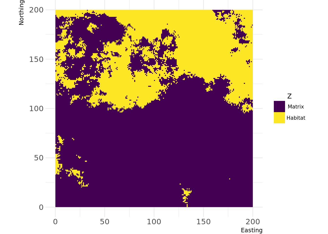
The following functions are implemented:

Utilities:

util_binarize: Binarize continuous raster values, if > 1 breaks are given, return a RasterBrick.
util_classify: Classify a raster into proportions based upon a vector of class weightings.
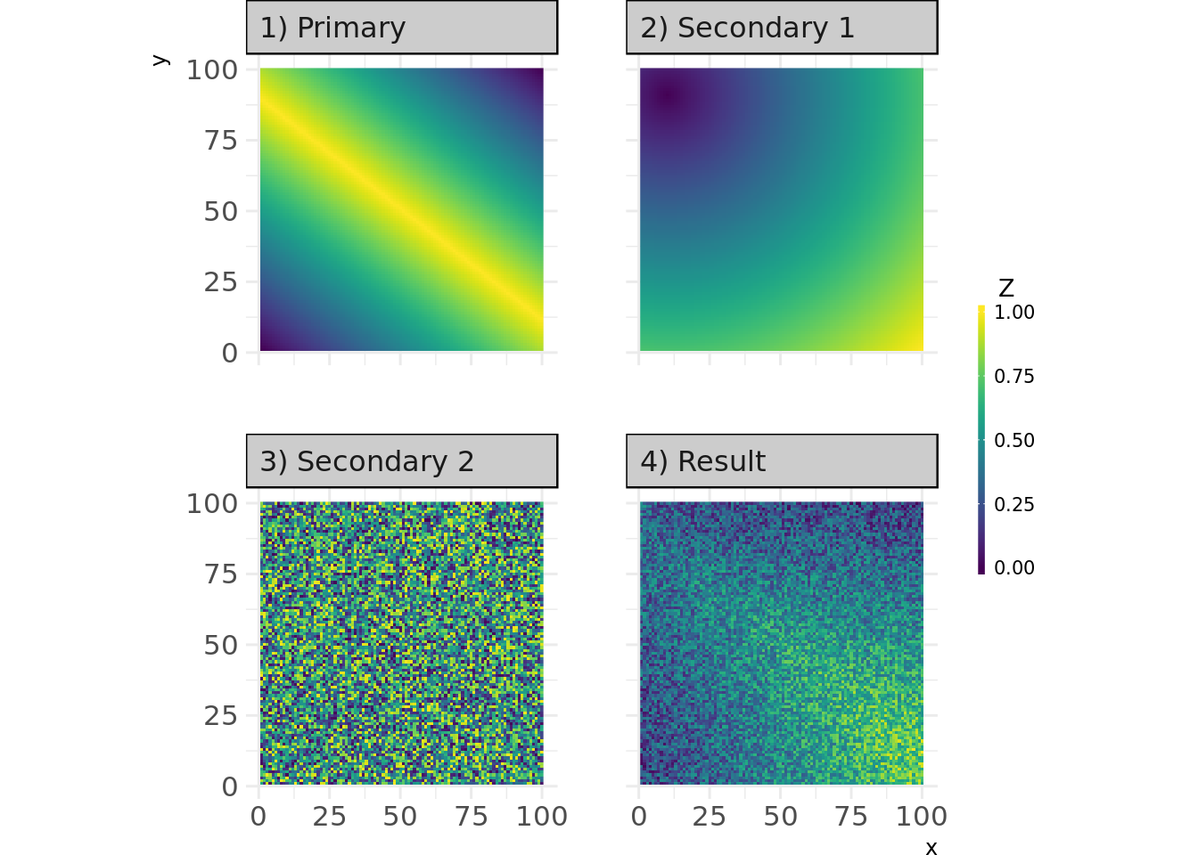
util_merge: Merge a primary raster with other rasters weighted by scaling factors.
util_raster2tibble, util_tibble2raster: Coerce raster* objects to tibbles and vice versa.
util_rescale: Linearly rescale element values in a raster to a range between 0 and 1.

Visualization

util_plot: Plot a Raster* object with the landscapetools default theme (as ggplot).
util_facetplot: Plot multiple raster (RasterStack, -brick or list of raster) side by side as facets.

Themes:

theme_nlm, theme_nlm_grey: Opinionated ggplot2 theme to visualize raster (continuous data).
theme_nlm_discrete,theme_nlm_grey_discrete: Opinionated ggplot2 theme to visualize raster (discrete data).
util_import_roboto_condensed: Import Roboto Condensed font for theme_nlm.

Installation

You can install the development version from GitHub with:

# install.packages("devtools")
devtools::install_github("marcosci/landscapetools")

Usage

library(nlmr)
library(landscapetools)
# Create an artificial landscape
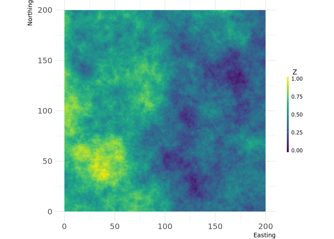
nlm_raster <- nlm_fbm(ncol = 200, nrow = 200, fract_dim = 0.8)
util_plot(nlm_raster)

Utilities

Binarize

# Binarize the map into habitat and matrix
binarized_raster <- util_binarize(nlm_raster, breaks = 0.31415)
util_plot(binarized_raster, discrete = TRUE)

Classify

# Classify the map into land uses
classified_raster <- util_classify(nlm_raster,
                                   c(0.5, 0.25, 0.25),
                                   level_names = c("Land Use 1", "Land Use 2", "Land Use 3"))
util_plot(classified_raster, discrete = TRUE)

Merge

# Create a primary and two secondary maps
prim <- nlm_edgegradient(ncol = 100, nrow = 100)

sec1 <- nlm_distancegradient(ncol = 100, nrow = 100,
                             origin = c(10, 10, 10, 10))

sec2 <- nlm_random(ncol = 100, nrow = 100)

# Merge all maps into one
merg <- util_merge(prim, c(sec1, sec2), scalingfactor = 1)

# Plot an overview
merge_vis <- list(
    "1) Primary" = prim,
    "2) Secondary 1" = sec1,
    "3) Secondary 2" = sec2,
    "4) Result" = merg
)
util_facetplot(merge_vis)

csim063/landscapetools