Python toolbox for helping to keep your data and analyses organized. The currently implemented analyses are tailored towards electrocorticographic data collected for the Restoring Active Memory (RAM) project, but the code is easily exended to other types of data.
Why use this toolbox? A large challenge when analyzing data is simply keeping your data and results organized. This toolbox provides convenient methods for loading data, saving data, loading results, and saving results, and it uses automatically generated file paths based on your analysis parameters to keep everything nicely organized on disk. It also provides a standardized pipeline for analyzing an experiment, in which raw data for a subject is loaded, possibly transformed in some way and saved, a specific analysis is applied to those data, and the results are then saved.
The fundamental unit of analysis is a subject, which is a single individual who participated in a specific experiment. When you create a subject, you also specify the analysis you are performing (in this case SubjectSMEAnalysis, a Subsequent Memory Analyis):
from miller_ecog_tools.subject import create_subject
subject = create_subject(task='FR1', subject='R1154D', montage=0, analysis_name='SubjectSMEAnalysis')
Where task indicates the name of the experiment performance, subject is subject identifier code, and montage is the "montage number" for a subject's electrode configuration (montage may not be applicable to all experiments). analysis_name is the name of the analysis class you to instantiate. If you don't enter an analysis_name, a list of possible analyses will be printed. Note that create_subject() is really just a tool to make it easier to create your subject with specific data and analysis methods, you could do that same thing with:
from miller_ecog_tools.SubjectLevel.Analyses.subject_SME import SubjectSMEAnalysis
subject = SubjectSMEAnalysis(task='FR1', subject='R1154D', montage=0)
SubjectSMEAnalysis is a subclass of the classes SubjectEEGData and SubjectAnalysisBase, and thus has access to their methods. SubjectEEGData is a subclass of SubjectDataBase that is specific to loading eeg data, and it has methods for loading, computing, and saving data. SubjectAnalysisBase has methods for loading, computing, and saving analysis results.
First, create a subject, as shown above. Then set the attributes of the data and analysis. In the case of analyses using SubjectEEGData, which loads eeg data and then performs spectral decomposition, you may set:
# whether to load bipolar pairs of electrodes or monopolar contacts
self.bipolar = True

# This will load eeg and compute the average reference before computing power. Recommended if bipolar = False.
self.mono_avg_ref = False

# the event `type` to filter the events to. This can be a string, a list of strings, or it can be a function
# that will be applied to the events. Function must return events dataframe.
self.event_type = ['WORD']

# power computation settings
self.start_time = -500
self.end_time = 1500
self.wave_num = 5
self.buf_ms = 2000
self.noise_freq = [58., 62.]
self.resample_freq = None
self.log_power = True
self.freqs = np.logspace(np.log10(1), np.log10(200), 8)
self.mean_over_time = True
self.time_bins = None
self.use_mirror_buf = False
So if I wanted to compute power starting at 0 ms and continuing until 2000 ms (relative to each event in .event_type) at 30 log-spaced frequencies between 1 and 200 Hz (leaving the other parameters the same) I would set:
subject.start_time = 0
subject.end_time = 2000
subject.freqs = np.logspace(np.log10(1), np.log10(200),30)
This would automatically set the save directory to the following path, based on the parameters:
/scratch/jfm2/python/FR1/30_freqs_1.000_200.000_bipol/0_start_2000_stop/1_bins/R1154D/0/power
And then load data (and save data):
subject.load_data()
subject.save_data()
After data is loaded, it is stored in .subject_data attribute.
With data loaded, you can run an analysis. SubjectSMEAnalysis has the following settable attributes:
# string to use when saving results files
self.res_str = 'sme.p'

# The SME analysis is a contract between two conditions (recalled and not recalled items). Set
# recall_filter_func to be a function that takes in events and returns indices of recalled items
self.recall_filter_func = None
.res_str is something that every analysis subclass should set on its own. It defines the name of the results file that will be saved. .recall_filter_func must a function that a returns a boolean of the good memory and bad memory events. For example:
def rec_func(subject_data):
    return subject_data.event.data['recalled'] == 1
subject.recall_filter_func = rec_func
Now run the analysis:
subject.analysis()and the results are accessible in subject.res dictionary. You can save the results with subject.save_res_data(), in this case saving to: /scratch/jfm2/python/FR1/30_freqs_1.000_200.000_bipol/0_start_2000_stop/1_bins/R1001P/0/SubjectSMEAnalysis_res/R1001P_sme.p
Running this all at once: Instead of all the above steps, there is a convenience function .run() to do it all for you. This produces the same results:
from miller_ecog_tools.subject import create_subject
subject = create_subject(task='FR1', subject='R1154D', montage=0, analysis_name='SubjectSMEAnalysis')

# set data parameters
subject.start_time = 0
subject.end_time = 2000
subject.freqs = np.logspace(np.log10(1), np.log10(200),30)

# set analyis parameters
def rec_func(subject_data):
    return subject_data.event.data['recalled'] == 1
subject.recall_filter_func = rec_func

# run it
subject.run()
This 1) loads/computes data, 2) can save data, 3) loads/computes results, and 4) can save results See the specific attributes in SubjectData and SubjectAnalysisBase for setting whether data should be load or computed or saved or not.
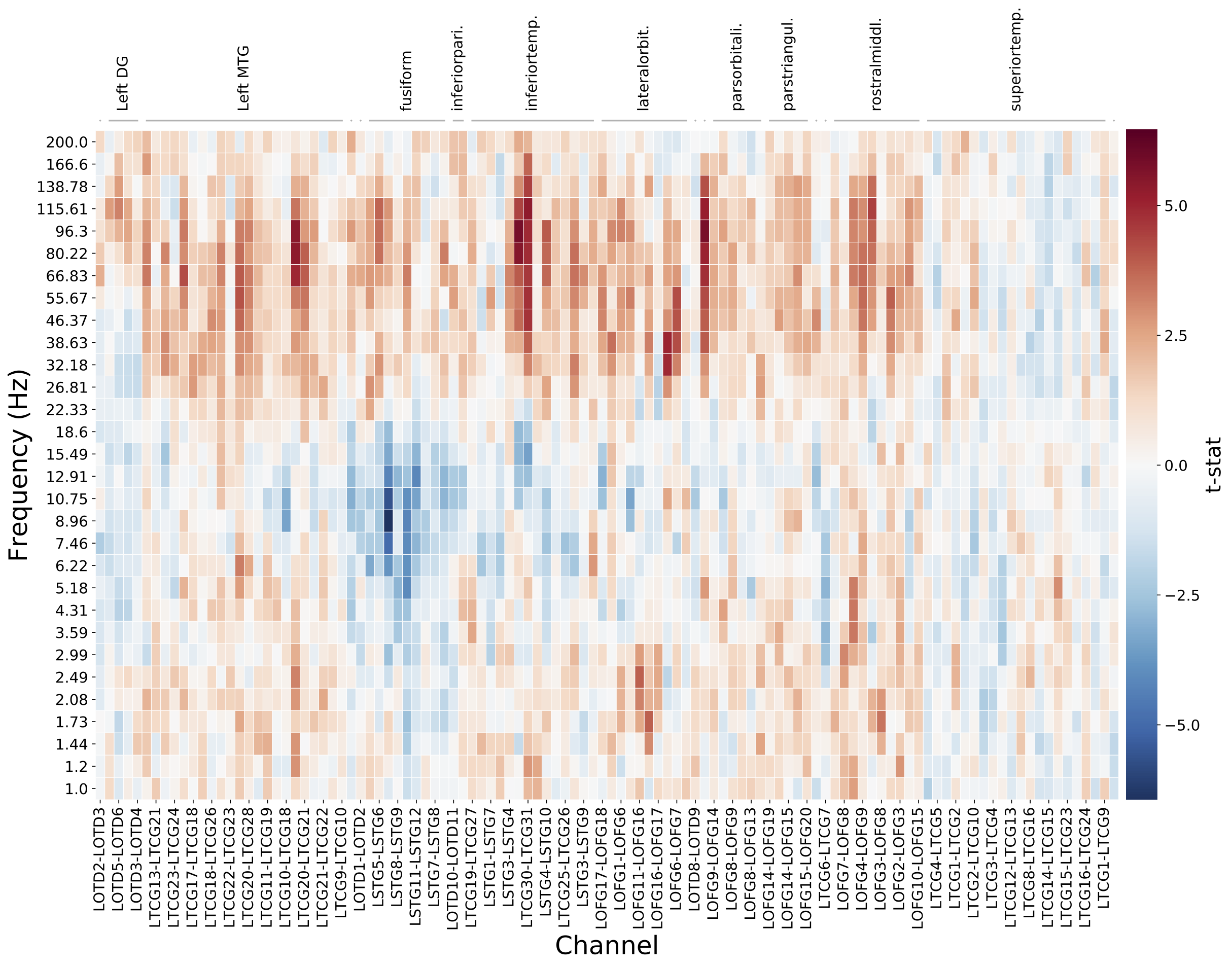
Because this toolbox is based on having a class for each analysis, it is also often very useful to create analysis specific methods in each class. This is good place for custom plotting functions. For example, SubjectSMEAnalysis has a custom plotting function for creating a heatmap of data from all electrodes, in this case sorting the columns by brain regions.
subject.plot_elec_heat_map(sortby_column1='stein.region', sortby_column2='ind.region')The prior SME analysis compared distributions of remembered and forgotten items using univariate t-tests. A slightly more complex analysis approach would be to specifically predict which items were remembered and forgotten using a cross-validated machine learning approach, in this case utilizing a penalized logistic regression. Because this analysis class (SubjectClassifierAnalysis) is a subclass of SubjectEEGData (just like SubjectSMEAnalysis), we can easily run the classifier on exactly the same data. See the class definition for additional settable parameters.
from miller_ecog_tools.subject import create_subject
subject = create_subject(task='FR1', subject='R1154D', montage=0, analysis_name='SubjectClassifierAnalysis')

# set data parameters
subject.start_time = 0
subject.end_time = 2000
subject.freqs = np.logspace(np.log10(1), np.log10(200),30)

# set analyis parameters
def rec_func(subject_data):
   return subject_data.event.data['recalled'] == 1
subject.recall_filter_func = rec_func

# run it
subject.run()
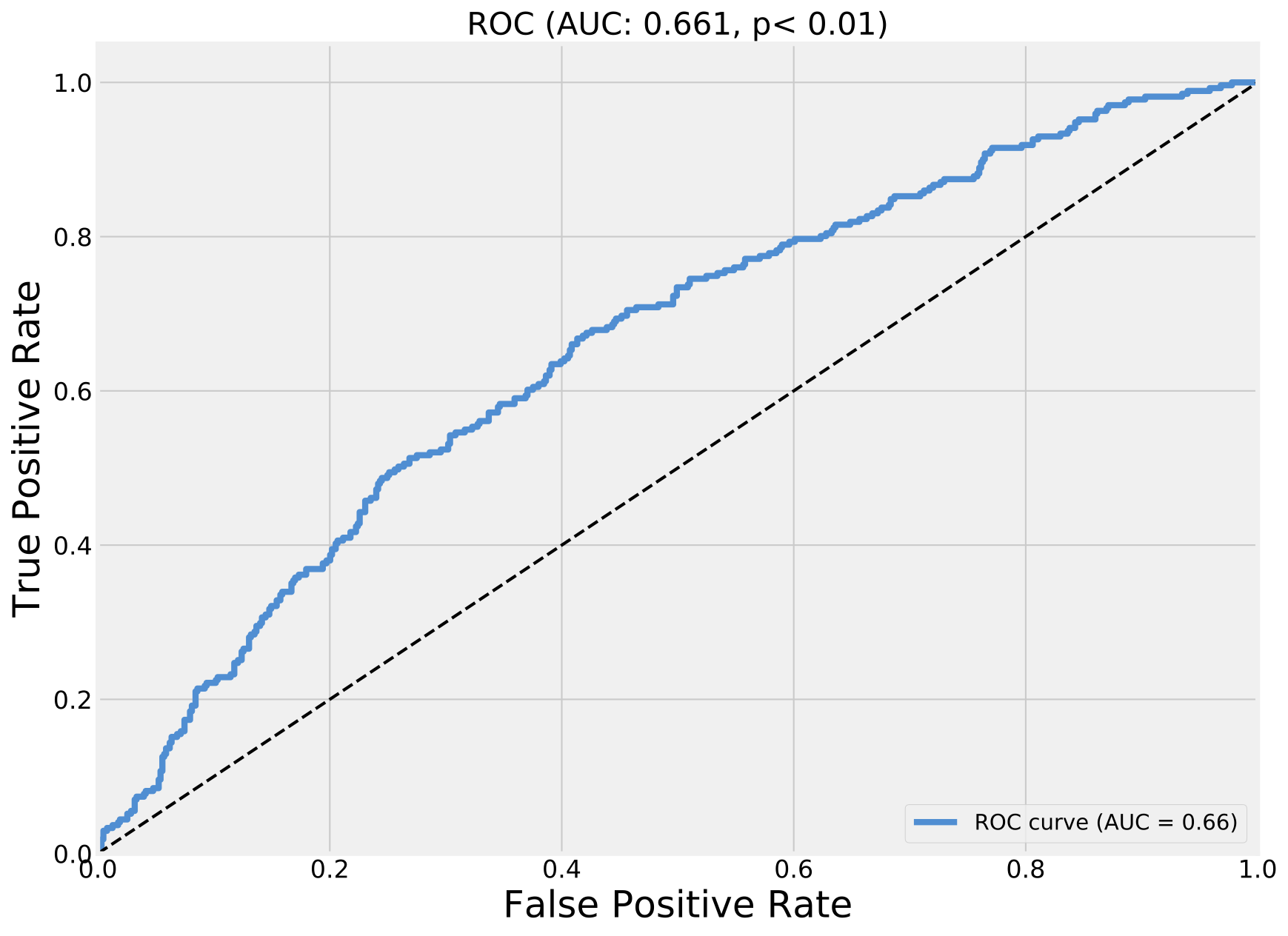
This analysis class has its own plotting functions as well, including a visualization of the classifier performance known as the ROC curve and it's associated metric, the Area Under the Curve (AUC).
subject.plot_roc()To create a new analysis, just add a new .py file to the SubjectLevel.Analyses directory with the following structure. The name of the class must end with Analysis in order for create_subject() to automatically know about it. The new analysis class should inherent from SubjectAnalysisBase and a subclass of SubjectData. Currently, the only option is SubjectEEGData. The class must have a _generate_res_save_path method and an analysis method. .analysis() should do computations on the data in self.subject_data and put the results in the self.res dictionary. Feel free to add any additional methods, like custom plots.
import os

from miller_ecog_tools.SubjectLevel.subject_analysis import SubjectAnalysisBase
from miller_ecog_tools.SubjectLevel.subject_eeg_data import SubjectEEGData


class NewAnalysis(SubjectAnalysisBase, SubjectEEGData):
    """
    Subclass of SubjectAnalysis and SubjectEEGData that does ........
    """

    def __init__(self, task=None, subject=None, montage=0):
        super(NewAnalysis, self).__init__(task=task, subject=subject, montage=montage)

        # string to use when saving results files
        self.res_str = 'new_save_string.p'

        # create any other analysis specific attributes here

    def _generate_res_save_path(self):
        self.res_save_dir = os.path.join(os.path.split(self.save_dir)[0], self.__class__.__name__+'_res')

    def analysis(self):
        """
        Do some analysis with the data in self.subject_data and put the results in the self.res dictionary.
        """
        if self.subject_data is None:
print('%s: compute or load data first with .load_data()!' % self.subject) While you could perform group level analyses by iterating over a list of subjects, running an analyses for each subject, and aggregating the results, this toolbox provides a convenient method for automatically performing this task, and it also provides a number of useful features.
Given a list of subjects and analyses parameters, the Group class will automatically run the specified analyses with the specified settings on each subject, it will automatically log any errors, it can create a parallel pool that can be used to parallize within subject computations, and lastly it can automatically make use of GroupLevel analyses for aiding in group statistics or plotting.
This code below processes every subject who completed the "FR1" experiment.
# import the group analysis module
from miller_ecog_tools.GroupLevel import group

# import the utility RAM_helpers, which is used to interact with our "RAM" dataset
# We will use it to load a dataframe of subjects who performed a specific experiemtn
from miller_ecog_tools.Utils import RAM_helpers

# load the dataframe of subjects and montage numbers
subj_montage = RAM_helpers.get_subjs_and_montages('FR1')

# define our function for labeling items as either remembered or forgotten
def rec_func(subject_data):
    return subject_data.event.data['recalled'] == 1

# create a dictionary of parameters we would like to set
kwargs = {'recall_filter_func': rec_func,
         'start_time': 0,
         'end_time': 2000,
         'mean_over_time': True,
         'freqs': np.logspace(np.log10(1), np.log10(200),30),
         'do_not_compute': True}

# initialize the group class, and then just call run!
res = group.Group(subject_montage=subj_montage, task='FR1', analysis_name='SubjectSMEAnalysis', **kwargs)
res.run()
Once complete, the class attribute subject_objs will be a list of all the subject objects that were processed, with their respective res dictionaries containing the subject specific results.
If you create a class in GroupLevel.Analysis with the same name as a subject level analysis, simply swapping out the word "Subject" with the word "Group" in the class name, then the class attribute group_helpers will be an instantiated version of that class. The only input to a group level analyis class is the list of subjects objects. You are then free to add any plotting or analysis code to this class that would be helpful.
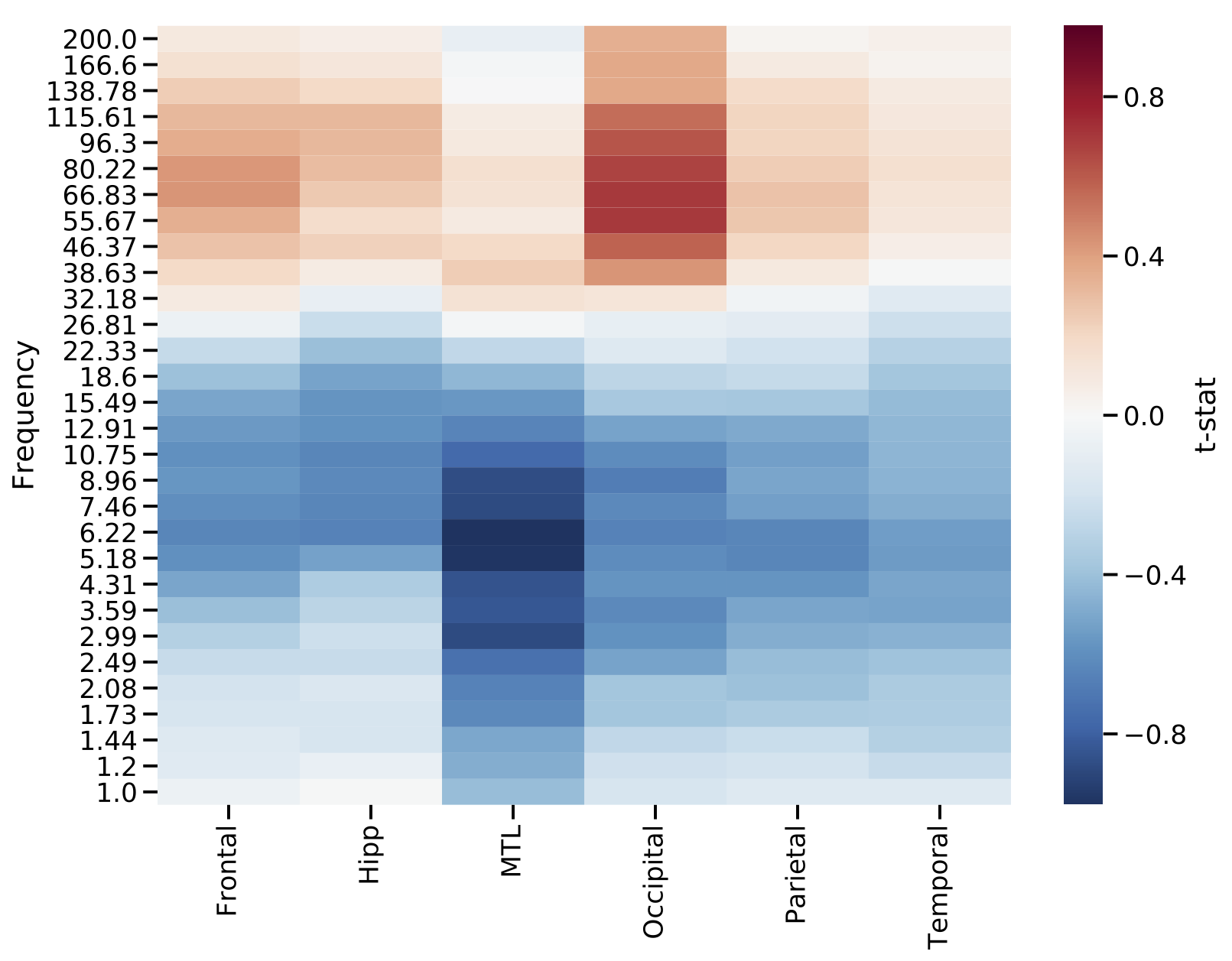
For example, GroupSME has a method for for visualizing the grand mean across subjects as a function of brain region and frequency. This result demonstrates that higher frequency activity tends to increase and lower frequency activity tends to decrease during successful encoding.
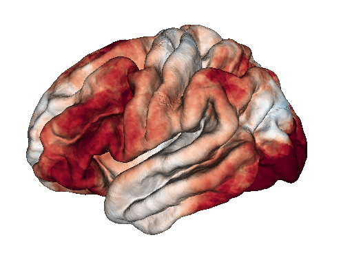
res.group_helpers.plot_region_heatmap()And there is also a function to visualize the results on a 3D rendered brain. Here, we are plotting the average result between 40 and 200 Hz, requiring an electrode to be within 12.5 mm of a vertex on the cortical surface in order for its data to be counted at that location.
res.group_helpers.plot_group_brain_activation(radius=12.5, freq_range=(40, 200), clim=1, cmap='RdBu_r')Different derived SubjectDataBase classes will likely need to interact with data on disk in different ways. SubjectEEGData works with data from the RAM project, and the utility Utils.RAM_helpers contains many functions for reading this paricular type of data. Utils should be expanded to contain helper functions for other types of data, when needed.


