Preface
Provided with datasets on home sales in Ames, Iowa from the years 2006-2010, the task given is to perform an exploratory data analysis determining the suitability of using a linear regression for prediction of Sale Price. A regression performed on the response variable Sale Price as explained by 23 predictor variables. The multiple linear regression model is then scrutinized to evaluate its suitability for use as a tool in prediction, and to identify which variables are significant predictors ranked by P-value and correlation. Sample predictions were performed on the first 20 occurrences of complete cases in the testing dataset. Summary statistics of the linear model result in an adjusted R-squared value of 0.84, and an R-value of 0.9 which is strong evidence that the model is an accurate and strong predictor of Sale Price. Overall Quality of the home had the greatest predictive power in explaining Sale Price. Technologies utilized for visualization and analysis include: RStudio, the base R-package, caret, dplyr, corrplot, and PerformanceAnalytics.
Data Summary
In preparation for data analysis the ID attribute was removed, and a combined data frame was created for the purposes of frequency comparison using histograms.
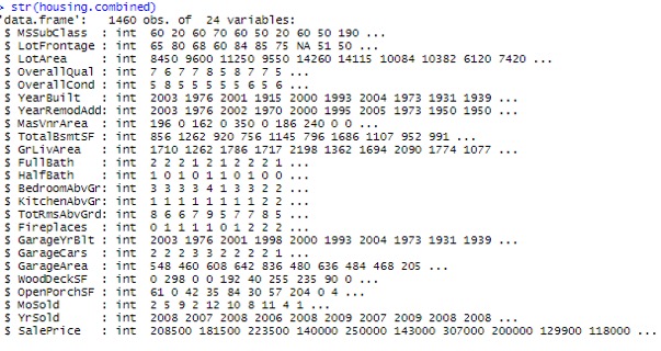
Figure 1 - R output for Structure of the combined dataset.
As shown in Figure 1, the training and testing data sets consist of 1000 and 460 observations of 24 variables. The datasets were imported into R using read.csv(), and all variables were assigned a numeric datatype by default. It was noted that the MSSubClass attribute is in fact a categorical factor with 16 levels. Substantial consideration was given in determining if modifying the type was necessary, a judgement was made that doing so would only complicate programming the model. Therefore, the int datatype was preserved. Later in the analysis it become apparent that this decision did not impact the accuracy of the linear model.
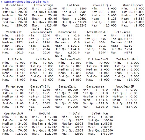
Figure 2 - R Summary statistics output for the training dataset.
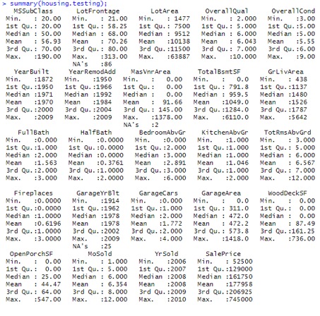
Figure 3 - R Summary statistics output for the testing set.
The summary statistics displayed in Figure 2 and Figure 3 were used to confirm homogeneity between the testing and training set prior to testing. It is important to observe the cases where the statistics output is meaningless, in this case, the obvious problem is with MSubClass. The narrow difference in the standard deviation of the response variable for each dataset, expressed by Figure 4, also supports their suitability for testing.
Figure 4 - R outputs for standard deviation for Sale Price.
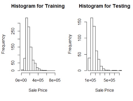
Figure 5 - Histograms of Sale Price for training and testing datasets.
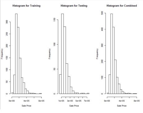
Figure 6 - Histograms for Sale Price for testing, training, and combined dataset for comparison.
Histogram obtained by the function shown in Figure 5 and Figure 6 visualize the frequency distribution of Sale Price. The similarities are quite remarkable, with minor variation. Compared, the three data assets all display a right skewed distribution and are a relatively uniform across data sets. Conclusively, the number of sales of lower priced homes is greater overall than that of higher priced homes. This behavior and skew can be explained by the fact that most people cannot afford to buy expensive houses.
Linear Regression Model
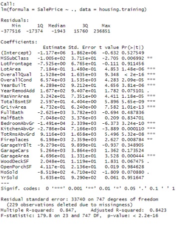
A linear regression was performed explaining the response variable Sale Price by all the other variables. Using linear regression and summary statistics, variables which are statistically significant predictors can be identified by their P-values.
Figure 7 - Multiple linear regression in R, Sale Price explained by all variables.
The summary statistics of the linear model also determine that R is significant. The P value annotated by asterisks in the summary output, shown in Figure 8, immediately reveal which variables have significant predictive capability. There are eleven variables with P values under the significance code level 0.001, annotated by *** : LotArea, OverallQual, OverallCond, YearBuilt, MasVnrArea, TotalBsmtSF, GrLivArea, BedroomAbvGrd, KitchenAbvGrd, TotalRmsAbvGrd, and GarageArea. All factors exhibit positive influence on Sale Price, (i.e.) as they increase, so does Sale Price.
The P value represents the probability of the correlation coefficient being attributed to variation. P values closer to zero are more significant predictors. The correlation coefficients are the measure of influence that each variable has in the prediction (slope of the regression line). A significance level of 0.001 interpreted as a 0.1% chance that the coefficient will be equal 0, (i.e.) we are 99% certain that it is significant.
Figure 8 - Summary of linear regression model for Sale Price as explained by all variables.
Correlation Plots
Figure 9 - R code used to generate correlation plots.
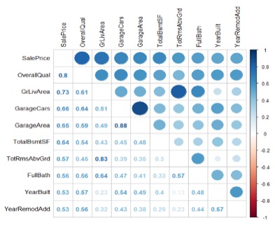
Using the R code in Figure 8, correlation plots are created to visualize the relationships between variables. Filtering was done by increasing the threshold of correlations that were plotted to select those with a correlation > 0.5 or 50% in Figure 11. This yielded 10 variables with the greatest correlation: OverallQual, GrLivArea, GarageCars, GarageArea, TotalBsmtSF, TotRmsAbvGrd, FullBath, YearBuilt, YearRemodAdd. Overall Quality is the strongest in both evaluations of P-Value and Correlation. The P value of Overall Quality < 2e^-16 is impressive.
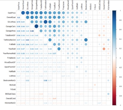
Figure 10 - Correlation Plot for all variables minus NAs.
Figure 11 - Correlation plot for variables with correlations > 0.5.
Prediction
Figure 12 - Predicting Sale Price from the first 20 complete cases of the testing dataset.
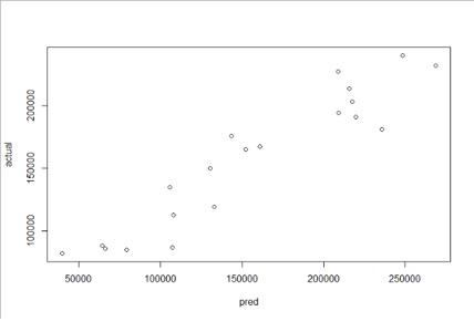
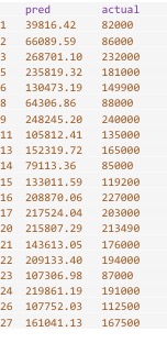
The predict function was used to calculate the response variable on a small testing sample. The scatter plot of predicted versus actual, shown in Figure 13, displays an obvious linear relationship with a positive and increasing slope. The linear relationship offers a strong visual representation of the model’s high precision, providing support of the use in prediction. A table of values plotted are provided in Figure 14. Comparing the result of difference between predicted and observed shows a narrow margin of error in most cases.
Figure 13 - Comparison scatter plot for predicted vs actual values.
Figure 14 - View of the comparison data frame containing predicted and actual values.
References
Berrier, J.,
Nestler, S., Pardoe, I., Sturdivant, R., &
Watts, K. (2018). ZyBook: Mis 470: Data
Science Foundations.
DSS - Interpreting Regression Output. (2007). Retrieved October 23,
2019, from https://dss.princeton.edu/online_help/analysis/interpreting_regression.htm.
Information Builders. (2018). Ebook. Explanation of the Regression Model WebFOCUS 8 Technical Library. Retrieved November 6, 2019, from https://infocenter.informationbuilders.com/wf80/index.jsp?topic=%2Fpubdocs%2FRStat16%2Fsource%2Ftopic41.htm
Karimi, M. (2017, August 2). RPubs - Regression Models - MPG vs AM analysis for mtcars dataset. . Retrieved November 6, 2019, from https://rpubs.com/mkarimi926/296145
W. N. Venables, D. M. Smith and the R Core Team. (2019). An Introduction to R [Epub] (R, version 3.6.1). Retrieved November 6, 2019, from https://cran.r-project.org/doc/manuals/r-release/R-intro.pdf
Appendix I - Variable Descriptions
MSSubClass: Identifies the type of dwelling involved in the sale.
20 1-STORY 1946 & NEWER ALL STYLES
30 1-STORY 1945 & OLDER
40 1-STORY W/FINISHED ATTIC ALL AGES
45 1-1/2 STORY - UNFINISHED ALL AGES
50 1-1/2 STORY FINISHED ALL AGES
60 2-STORY 1946 & NEWER
70 2-STORY 1945 & OLDER
75 2-1/2 STORY ALL AGES
80 SPLIT OR MULTI-LEVEL
85 SPLIT FOYER
90 DUPLEX - ALL STYLES AND AGES
120 1-STORY PUD (Planned Unit Development) - 1946 & NEWER
150 1-1/2 STORY PUD - ALL AGES
160 2-STORY PUD - 1946 & NEWER
180 PUD - MULTILEVEL - INCL SPLIT LEV/FOYER
190 2 FAMILY CONVERSION - ALL STYLES AND AGES
LotFrontage: Linear feet of street connected to property
LotArea: Lot size in square feet
OverallQual: Rates the overall material and finish of the house
10 Very Excellent
9 Excellent
8 Very Good
7 Good
6 Above Average
5 Average
4 Below Average
3 Fair
2 Poor
1 Very Poor
OverallCond: Rates the overall condition of the house
10 Very Excellent
9 Excellent
8 Very Good
7 Good
6 Above Average
5 Average
4 Below Average
3 Fair
2 Poor
1 Very Poor
YearBuilt: Original construction date
YearRemodAdd: Remodel date (same as construction date if no remodeling or additions)
MasVnrArea: Masonry veneer area in square feet
TotalBsmtSF: Total square feet of basement area
GrLivArea: Above grade (ground) living area square feet
FullBath: Full bathrooms above grade
HalfBath: Half baths above grade
BedroomAbvGr: Bedrooms above grade (does NOT include basement bedrooms)
KitchenAbvGr: Kitchens above grade
TotRmsAbvGrd: Total rooms above grade (does not include bathrooms)
Fireplaces: Number of fireplaces
GarageYrBlt: Year garage was built
GarageCars: Size of garage in car capacity
GarageArea: Size of garage in square feet
WoodDeckSF: Wood deck area in square feet
OpenPorchSF: Open porch area in square feet
MoSold: Month Sold (MM)
YrSold: Year Sold (YYYY)
Special Thanks to Kaggle Member Erik Bruin for his providing these in his report on the original data set. https://www.kaggle.com/erikbruin/house-prices-lasso-xgboost-and-a-detailed-eda/report
