The project is based around the SegTHOR challenge data, which was kindly allowed by Caroline Petitjean (challenge organizer) to use for the course. The challenge was originally on the segmentation of different organs: heart, aorta, esophagus and trachea.
This codebase is given as a starting point, to provide an initial neural network that converges during training. (For broader context, this is itself a fork of an older conference tutorial we gave few years ago.) It also provides facilities to locally run some test on a laptop, with a toy dataset and dummy network.
Summary of codebase (in PyTorch)
- slicing the 3D Nifti files to 2D
.png; - stitching 2D
.pngslices to 3D volume compatible with initial nifti files; - basic 2D segmentation network;
- basic training and printing with cross-entroly loss and Adam;
- partial cross-entropy alternative as a loss (to disable one class during training);
- debug options and facilities (cpu version, "dummy" network, smaller datasets);
- saving of predictions as
.png; - log the 2D DSC and cross-entropy over time, with basic plotting;
- tool to compare different segmentations (
viewer/viewer.py).
Some recurrent questions might be addressed here directly. As such, it is expected that small change or additions to this readme to be made.
In the following, a line starting by $ usually means it is meant to be typed in the terminal (bash, zsh, fish, ...), whereas no symbol might indicate some python code.
git clone https://github.com/danilotpnta/ai4mi_project.git
cd ai4mi_project
git submodule init
git submodule update
This codebase was written for a somewhat recent python (3.10 or more recent). (Note: Ubuntu and some other Linux distributions might make the distasteful choice to have python pointing to 2.+ version, and require to type python3 explicitly.) The required packages are listed in requirements.txt and a virtual environment can easily be created from it through pip:
python -m venv ai4mi
source ai4mi/bin/activate
which python  # ensure this is not your system's python anymore
python -m pip install -r requirements.txt
Conda is an alternative to pip, but is recommended not to mix conda install and pip install.
The synthetic dataset is generated randomly, whereas for Segthor it is required to put the file segthor_train.zip (required a UvA account) in the data/ folder. If the computer running it is powerful enough, the recipe for data/SEGTHOR can be modified in the Makefile to enable multi-processing (-p -1 option, see python slice_segthor.py --help or its code directly).
make data/TOY2
make data/SEGTHOR
For windows users, you can use the following instead
$ rm -rf data/TOY2_tmp data/TOY2
$ python gen_two_circles.py --dest data/TOY2_tmp -n 1000 100 -r 25 -wh 256 256
$ mv data/TOY2_tmp data/TOY2

$ sha256sum -c data/segthor_train.sha256
$ unzip -q data/segthor_train.zip

$ rm -rf data/SEGTHOR_tmp data/SEGTHOR
$ python  slice_segthor.py --source_dir data/segthor_train --dest_dir data/SEGTHOR_tmp \
         --shape 256 256 --retain 10
$ mv data/SEGTHOR_tmp data/SEGTHOR
The data can be viewed in different ways:
- looking directly at the
.pngin the sliced folder (data/SEGTHOR); - using the provided "viewer" to compare segmentations (see below);
- opening the Nifti files from
data/segthor_trainwith 3D Slicer or ITK Snap.
Running a training
$ python main.py --help
usage: main.py [-h] [--epochs EPOCHS] [--dataset {TOY2,SEGTHOR}] [--mode {partial,full}] --dest DEST [--gpu] [--debug]

options:
  -h, --help            show this help message and exit
  --epochs EPOCHS
  --dataset {TOY2,SEGTHOR}
  --mode {partial,full}
  --dest DEST           Destination directory to save the results (predictions and weights).
  --gpu
  --debug               Keep only a fraction (10 samples) of the datasets, to test the logic around epochs and logging easily.
$ python -O main.py --dataset SEGTHOR --model_name ENet --mode full
The codebase uses a lot of assertions for control and self-documentation, they can easily be disabled with the -O option (for faster training) once everything is known to be correct (for instance run the previous command for 1/2 epochs, then kill it and relaunch it):
python -O main.py --dataset SEGTHOR --model_name ENet --mode full
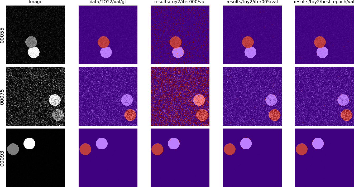
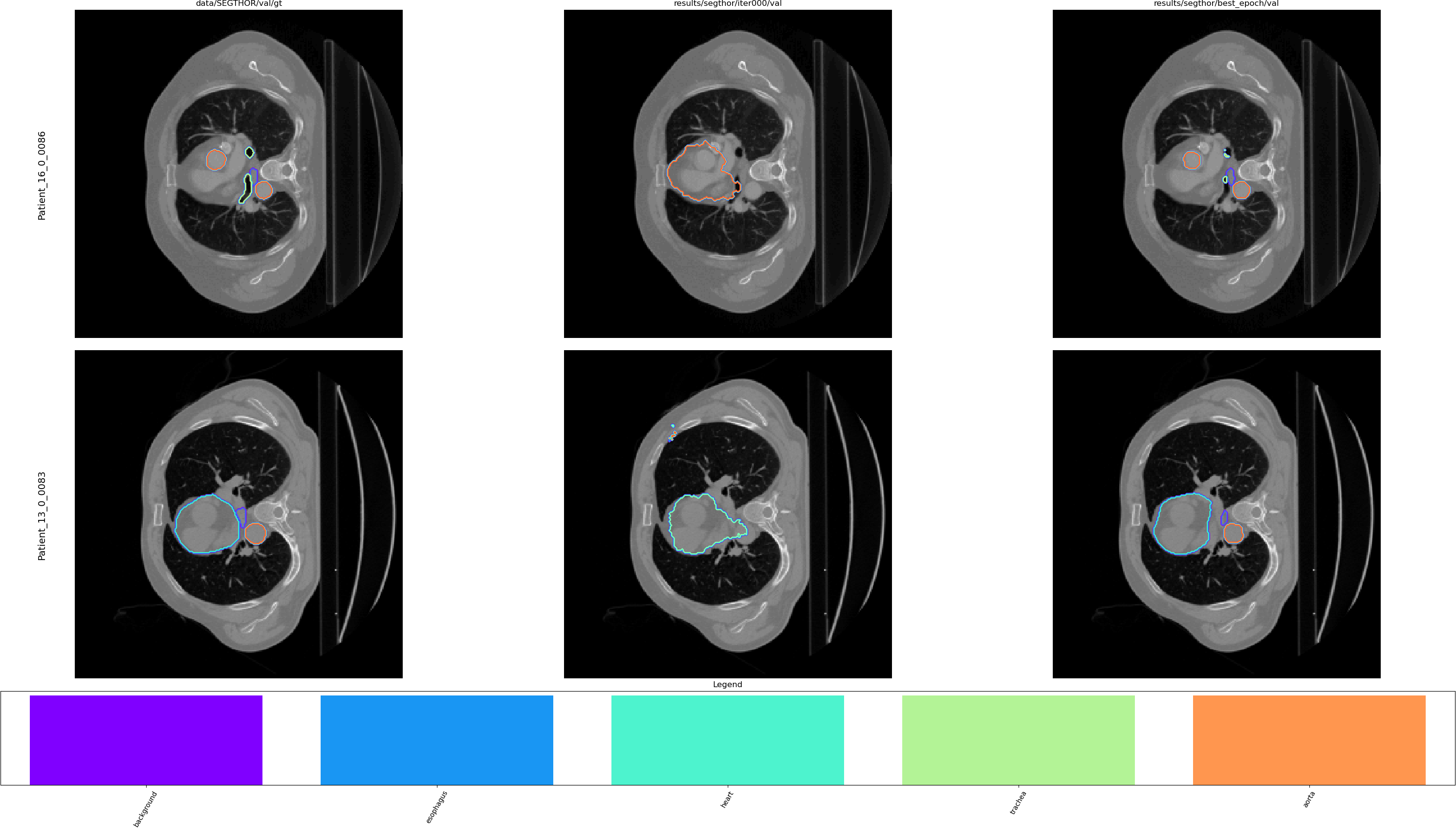
Comparing some predictions with the provided viewer (right-click to go to the next set of images, left-click to go back):
$ python viewer/viewer.py --img_source data/TOY2/val/img \
                                       data/TOY2/val/gt  \
                                       results/toy2/ce/iter000/val \
                                       results/toy2/ce/iter005/val \
                                       results/toy2/ce/best_epoch/val \
    --show_img -C 256 --no_contour
Note: if using it from a SSH session, it requires X to be forwarded (Unix/BSD, Windows) for it to work. Note that X forwarding also needs to be enabled on the server side.
$ python viewer/viewer.py --img_source data/SEGTHOR/val/img \
                                       data/SEGTHOR/val/gt \
                                       results/segthor/ce/iter000/val \
                                       results/segthor/ce/best_epoch/val \
    -n 2 -C 5 --remap "{63: 1, 126: 2, 189: 3, 252: 4}" \
    --legend --class_names background esophagus heart trachea aorta
To look at the results in 3D, it is necessary to reconstruct the 3D volume from the individual 2D predictions saved as images.
To stitch the .png back to a nifti file:
$ python stitch.py --data_folder results/segthor/ce/best_epoch/val \
    --dest_folder volumes/segthor/ce \
    --num_classes 255 --grp_regex "(Patient_\d\d)_\d\d\d\d" \
    --source_scan_pattern "data/segthor_train/train/{id_}/GT.nii.gz"
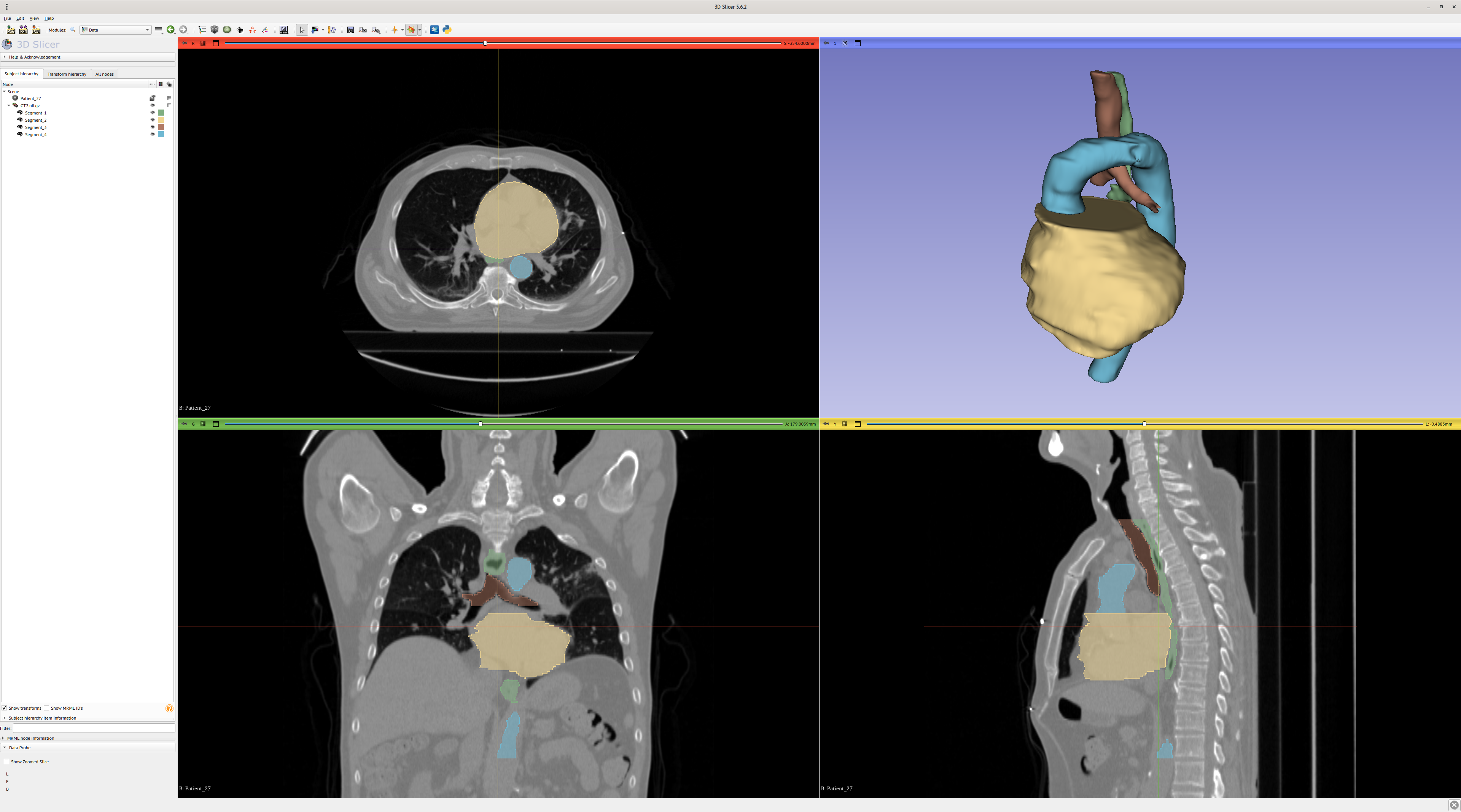
3D Slicer and ITK Snap are two popular viewers for medical data, here comparing GT.nii.gz and the corresponding stitched prediction Patient_01.nii.gz:
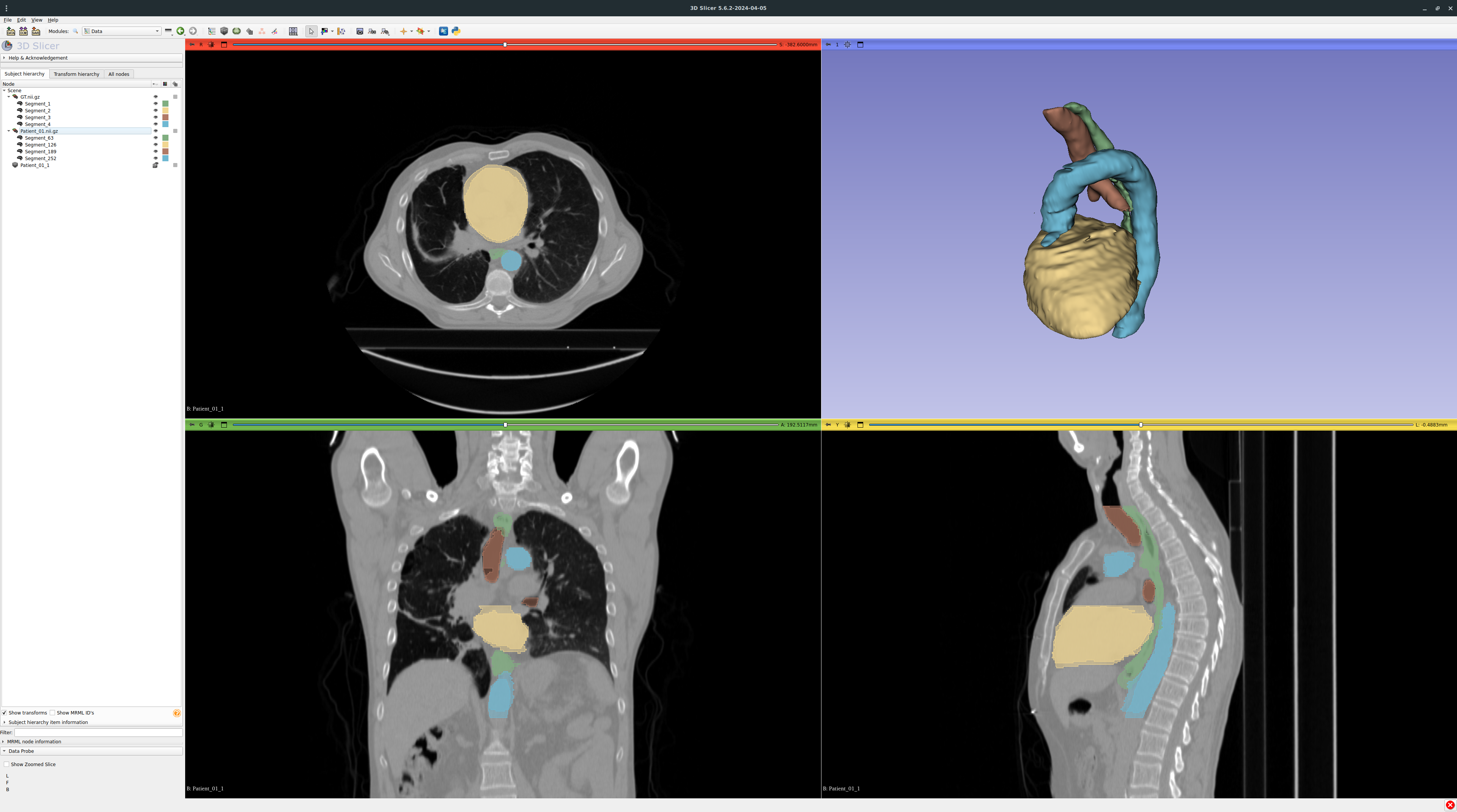
Zooming on the prediction with smoothing disabled:
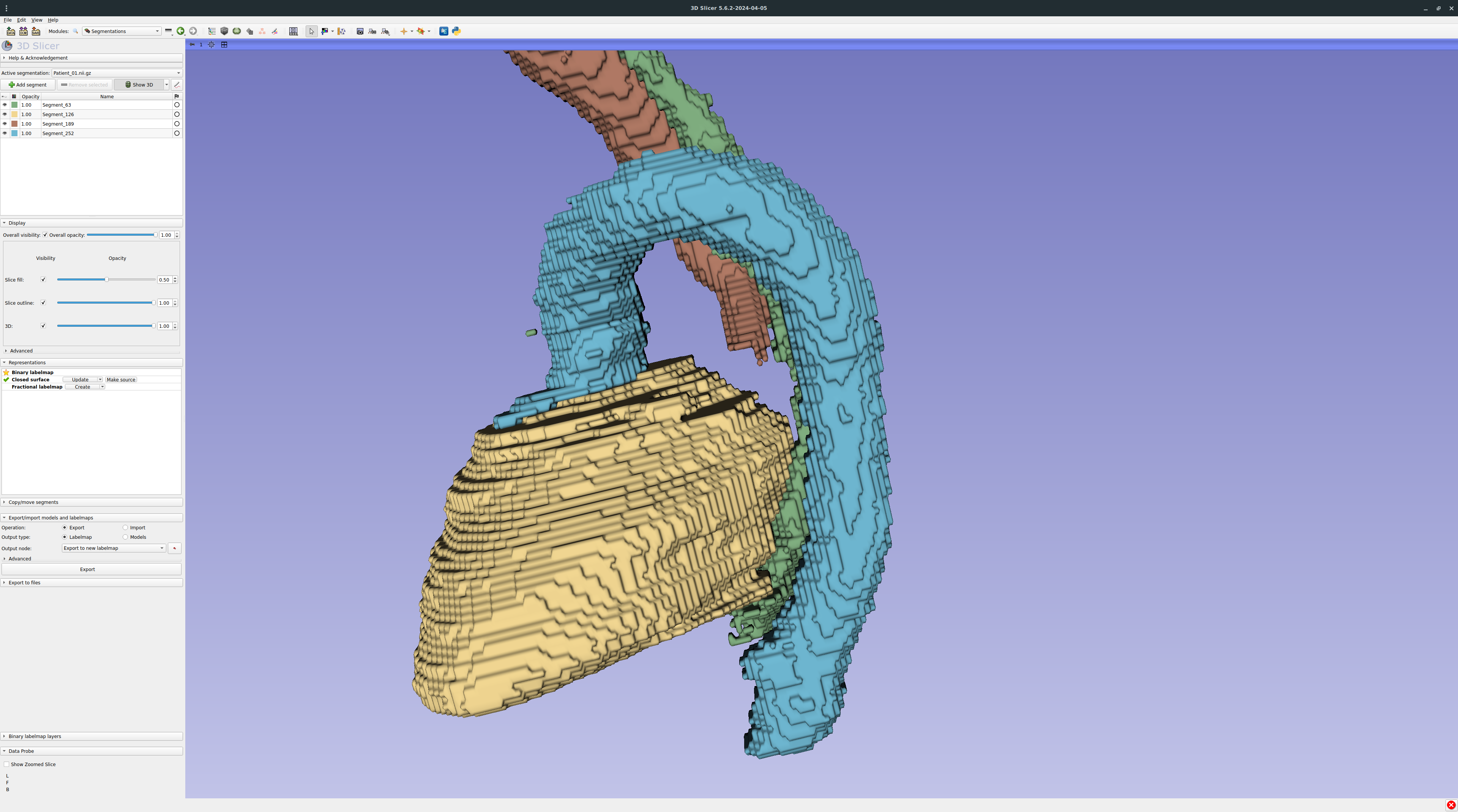
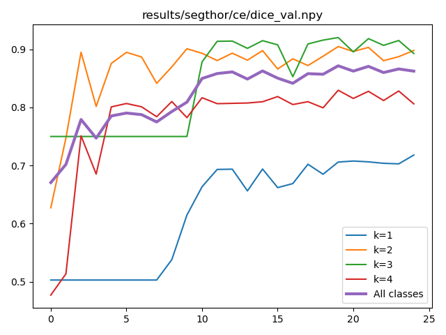
There are some facilities to plot the metrics saved by main.py:
$ python plot.py --help
usage: plot.py [-h] --metric_file METRIC_MODE.npy [--dest METRIC_MODE.png] [--headless]

Plot data over time

options:
  -h, --help            show this help message and exit
  --metric_file METRIC_MODE.npy
                        The metric file to plot.
  --dest METRIC_MODE.png
                        Optional: save the plot to a .png file
  --headless            Does not display the plot and save it directly (implies --dest to be provided.
$ python plot.py --metric_file results/segthor/ce/dice_val.npy --dest results/segthor/ce/dice_val.png
Plotting and visualization ressources:
Groups will have to submit:
- archive of the git repo with the whole project, which includes:
- pre-processing;
- training;
- post-processing where applicable;
- inference;
- metrics computation;
- script fixing the data using the matrix
AFFfromaffine.py(or rather its inverse); - (bonus) any solution fixing patient27 without recourse to
affine.py; - (bonus) any (even partial) solution fixing the whole dataset without recourse to
affine.py;
- the best trained model;
- predictions on the test set (
sha256sum -c data/test.zip.sha256as optional checksum); - predictions on the group's internal validation set, the labels of their validation set, and the metrics they computed.
The main criteria for scoring will include:
- improvement of performances over baseline;
- code quality/clear git use;
- the choice of metrics (they need to be in 3D);
- correctness of the computed metrics (on the validation set);
- (part of the report) clear description of the method;
- (part of the report) clever use of visualization to report and interpret your results;
- report;
- presentation.
The (bonus) lines give extra points, that can ultimately compensate other parts of the project/quizz.
$ git bundle create group-XX.bundle master
torch.save(net, args.dest / "bestmodel-group-XX.pkl")
All files should be grouped in single folder with the following structure
group-XX/
    test/
        pred/
            Patient_41.nii.gz
            Patient_42.nii.gz
            ...
    val/
        pred/
            Patient_21.nii.gz
            Patient_32.nii.gz
            ...
        gt/
            Patient_21.nii.gz
            Patient_32.nii.gz
            ...
        metric01.npy
        metric02.npy
        ...
    group-XX.bundle
    bestmodel-group-XX.pkl
The metrics should be numpy ndarray with the shape NxKxD, with N the number of scan in the subset, K the number of classes (5, including background), and D the eventual dimensionality of the metric (can be simply 1).
The folder should then be tarred and compressed, e.g.:
tar cf - group-XX/ | zstd -T0 -3 > group-XX.tar.zst
tar cf group-XX.tar.gz - group-XX/
Some installs (probably due to Python/Pytorch version mismatch) throw an error about an inability to pickle lambda functions (at the dataloader stage). Short of reinstalling everything, setting the number of workers to 0 seems to get around the problem (--num_workers 0).
It may happen that Pytorch, when installed through pip, was compiled for Numpy 1.x, which creates some inconsistencies. Downgrading Numpy seems to solve it: pip install --upgrade "numpy<2"
Windows has different paths names (\ in stead of /), so the default regex in the viewer needs to be changed to --id_regex=".*\\\\(.*).png".
