Time Series Decomposition

Introduction

Previously, you saw how we can combine several techniques to detrend our time series. Before we move on to our time series models, let's look at another method to remove trend and seasonality, names Decomposition.

Let's once again import the passengers dataset and the stationarity_check() function from previous to use time series decomposition and its effect on detrending a time series.

Objectives

You will be able to:

Understand what Time Series Decomposition is

Import our code

import pandas as pd
from pandas import Series
import numpy as np

import matplotlib.pylab as plt
%matplotlib inline

# Import the check_stationarity function from previous lab
def stationarity_check(TS):
    
    # Import adfuller
    from statsmodels.tsa.stattools import adfuller
    
    # Calculate rolling statistics
    rolmean = TS.rolling(window = 8, center = False).mean()
    rolstd = TS.rolling(window = 8, center = False).std()
    
    # Perform the Dickey Fuller Test
    dftest = adfuller(TS['#Passengers']) # change the passengers column as required 
    
    #Plot rolling statistics:
    fig = plt.figure(figsize=(12,6))
    orig = plt.plot(TS, color='blue',label='Original')
    mean = plt.plot(rolmean, color='red', label='Rolling Mean')
    std = plt.plot(rolstd, color='black', label = 'Rolling Std')
    plt.legend(loc='best')
    plt.title('Rolling Mean & Standard Deviation')
    plt.show(block=False)
    
    # Print Dickey-Fuller test results
    print ('Results of Dickey-Fuller Test:')

    dfoutput = pd.Series(dftest[0:4], index=['Test Statistic','p-value','#Lags Used','Number of Observations Used'])
    for key,value in dftest[4].items():
        dfoutput['Critical Value (%s)'%key] = value
    print (dfoutput)
    
    return None

# Import passengers.csv and set it as a time-series object. Plot the TS
data = pd.read_csv('passengers.csv')
ts = data.set_index('Month')
ts.index = pd.to_datetime(ts.index)
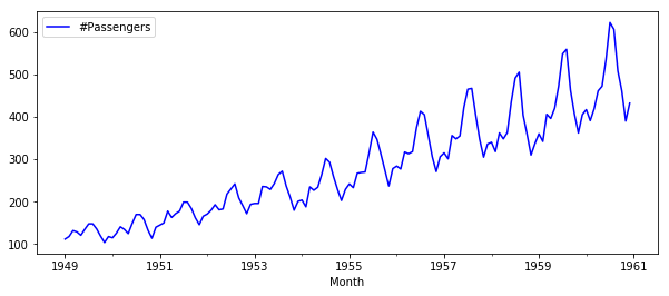
ts.plot(figsize=(10,4), color="blue");

Decomposing

Time series decomposition is a mathematical procedure which transforms a time series into multiple different time series. The original time series is often split into 3 component series:

Seasonal: Patterns that repeat with a fixed period of time. For example, a website might receive more visits during weekends; this would produce data with a seasonality of 7 days.

Trend: The underlying trend of the metrics. A website increasing in popularity should show a general trend that goes up.

Random: Also call “noise”, “irregular” or “remainder,” this is the residuals of the original time series after the seasonal and trend series are removed.

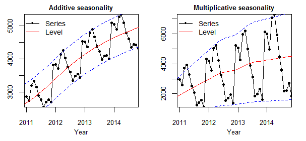
Additive or Multiplicative Decomposition?

To achieve successful decomposition, it is important to choose between the additive and multiplicative models, which requires analyzing the series. For example, does the magnitude of the seasonality increase when the time series increases?

Fortunately, statsmodels provides the convenient seasonal_decompose function to perform such decomposition out of the box. Details of this function are available here.

Let's use this function to perform following tasks:

Import seasonal_decompose from statsmodels.
Apply seasonal_decompose to log transformed TS.
Plot the trend, seasonality and residual.

# import seasonal_decompose
from statsmodels.tsa.seasonal import seasonal_decompose
decomposition = seasonal_decompose(np.log(ts))

# Gather the trend, seasonality and noise of decomposed object
trend = decomposition.trend
seasonal = decomposition.seasonal
residual = decomposition.resid

# Plot gathered statistics
plt.figure(figsize=(12,8))
plt.subplot(411)
plt.plot(np.log(ts), label='Original', color="blue")
plt.legend(loc='best')
plt.subplot(412)
plt.plot(trend, label='Trend', color="blue")
plt.legend(loc='best')
plt.subplot(413)
plt.plot(seasonal,label='Seasonality', color="blue")
plt.legend(loc='best')
plt.subplot(414)
plt.plot(residual, label='Residuals', color="blue")
plt.legend(loc='best')
plt.tight_layout()

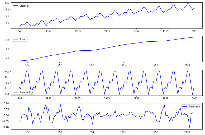
Here we can see that the trend, seasonality are separated out from data and we can model the residuals.

Using time-series decomposition makes it easier to quickly identify a changing mean or variation in the data. The plot above clearly shows the upwards trend of our data, along with its yearly seasonality. These can be used to understand the structure of our time-series. The intuition behind time-series decomposition is important, as many forecasting methods build upon this concept of structured decomposition to produce forecasts.

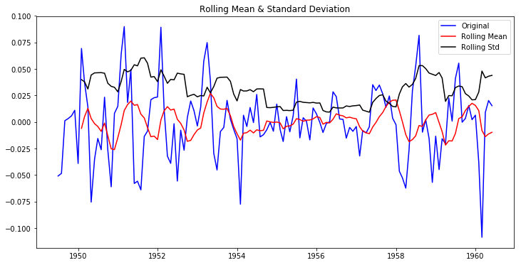
Lets check stationarity of residuals using our check_stationarity() function.

NOTE: drop NaN values first.

# Drop NaN values from residuals.
ts_log_decompose = residual
ts_log_decompose.dropna(inplace=True)

# Check stationarity
stationarity_check(ts_log_decompose)

Results of Dickey-Fuller Test:
Test Statistic                -6.332387e+00
p-value                        2.885059e-08
#Lags Used                     9.000000e+00
Number of Observations Used    1.220000e+02
Critical Value (1%)           -3.485122e+00
Critical Value (5%)           -2.885538e+00
Critical Value (10%)          -2.579569e+00
dtype: float64

The Dickey-Fuller test statistic is significant and very well below a (strict) 0.01 mark. So it seems reasonable to assume this time series is stationary.

Additional resources

We strongly recommend you to read this blogpost on decomposing time series!

Summary

In this lesson, we saw how to remove both trend and seasonality from a time-series using time series decomposition. We saw how decoposition allows us to better model the time-series for further analysis. you are now ready to perform predictive analyses and modeling with time-series data!

danjizquierdo/dsc-3-25-09-time-series-decomposition-nyc-ds-career-012819