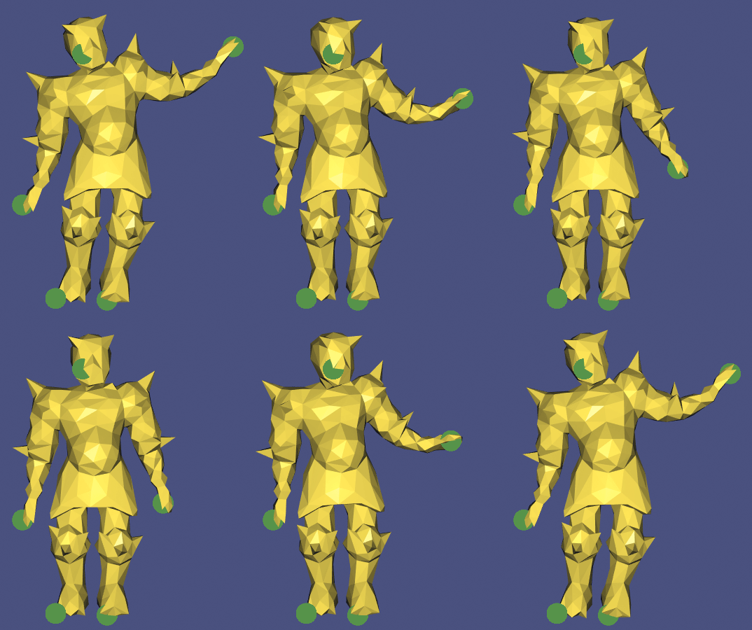
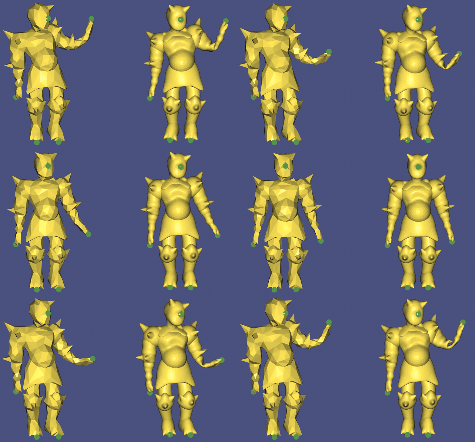
Geometry Processing – Deformation
To get started: Fork this repository then issue
git clone --recursive http://github.com/[username]/geometry-processing-deformation.git
Installation, Layout, and Compilation
See introduction.
Execution
Once built, you can execute the assignment from inside the build/ by running
on a given mesh:
./deformation [path to mesh.obj]
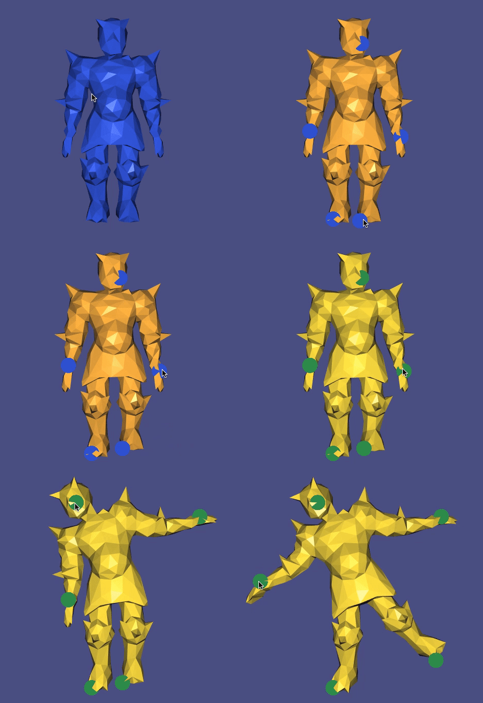
When the mesh is blue, the system is in "place handles" mode. Click on the mesh
to select vertex locations for control point handles. After pressing space to switch to
deformation mode, drag the handles. Pressing m will switch between different
deformation methods.
Background
In this assignment we explore smooth deformation of an existing shape. Shape deformation has many applications in geometry process; we will focus on interactive handle-based deformation. In this setup, the user repositions a sparse set of points and the goal is to propagate the transformation at these "handles" to the rest of the shape. To be interactive we should aim for computing the new deformation of the shape at around 30 frames per second.
Shape deformation is the transformation from its rest shape to a
new/current/deformed shape. If the position of a point on some 3D rest shape
given by
The propagation of the handles' deformation can be thought of in two complementary ways:
- as a scattered data interpolation problem, where handles provide sparse samples of an unknown displacement field, or
- as a shape optimization problem, where we try to define a new shape that retains the details of the old shape but fulfills the handle constraints.
In the following discussion we will take advantage of the ability to switch
between thinking of the unknowns as the positions of the deformed shape (
Continuity
We will limit ourselves to continuous deformations of shapes. That is, the shape will not tear, crack or change its topological features.
If we represent our shape discretely as a triangle
mesh (e.g., with rest vertices
in
Generic Distortion Minimization
A rest surface
\[ \hat{\x}(u,v) ∈ \R³. \]
Similarly the deformed surface can be represented as a position function
For the handle-based deformation problem we would like to find a new surface
(defined by
- adds as little distortion as possible to the shape, and
- satisfies the users constraints at selected handle positions.
We can cast this as an energy optimization problem. Suppose we have
energy functional
\[ \min_\x E(\x). \]
To ensure that the user's
\[
\text{ subject to } \x(u_i, v_i) = \g_i \ ∀ i = {1, … , k},
\]
where
While the constraints are straightforward, we have many choices for how to
formulate the energy function
\[ \min_\x ∫_Ω ‖ e(\x) ‖² \ dA \quad \text{ subject to } \x(u_i, v_i) = \g_i \ ∀ i = {1, … , k}, \]
where
Linear Methods
If we assume that the deformation between the rest shape given by
Gradient-based energy
Let us first consider minimizing the integral of squared variation of the displacement field:
\[
\min_\d ∫_Ω ‖ ∇\d ‖_F^2 \ dA \quad \text{ subject to } \d_i =
\g_i-\hat{\x}_i \ ∀ i = {1, … , k},
\]
where
$∇\d = \left(\begin{array}{ccc}
\frac{∂d^x}{∂u} & \frac{∂d^y}{∂u} & \frac{∂d^z}{∂u} \
\frac{∂d^x}{∂v} & \frac{∂d^y}{∂v} & \frac{∂d^z}{∂v}
\end{array}\right)$
the Jacobian
matrix of the displacement field
Deformation Gradient
If
$\I ∈ \R^{3 × 3}$ is the identity matrix, then the quantity$\F := \I + ∇\d$ is referred to as the deformation gradient in the mechanics community.
This is simply the familiar Dirichlet energy applied to each coordinate function of the displacement field independently.
We can discretize this over our triangle mesh surface the same way we have in smoothing and parameterization assignments:
\[
\min_{\D} \tr{\D^\transpose \L \D} \quad \text{subject to } \D_\text{handles} =
\g_\text{handles} - \hat{\V}\text{handles},
\]
where the rows of $\g\text{handles} ∈ \R^{k × 3}$ contains the new positions
of the
While easy to implement, this method suffers from a couple immediate problems:
- it is not smooth at constraints, and
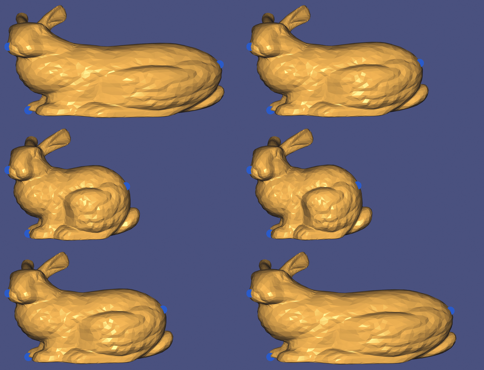
- then influence of handles dies off too quickly.
By minimizing the Dirichlet energy, each coordinate of "displacement field" is a harmonic function. Intuitively (however abstractly) we can think of each function as diffusing the user's constraints as if they were heat values. As such, each function diffuses quickly to an average, slowly varying value over most of the domain. As a displacement field a constant value for each coordinate function would mean a translation: most of the shape is simply translated.
The gradient operator (
\[
\min_\d ∫_Ω ‖ ∇\d ‖F^2 \ dA ⇒
\min\x ∫_Ω ‖ ∇(\x - \hat{\x}) ‖F^2 \ dA ⇒
\min\x ∫_Ω ‖ \underbrace{∇\x}\text{after} -
\underbrace{∇\hat{\x}}\text{before} ‖_F^2 \ dA.
\]
If we think of the gradient of the position function
Unfortunately, the gradient of the position function
Laplacian-based energy
If we model distortion as the change in a local feature descriptor, then a natural local and relative descriptor would be one that compared the position of some point on the shape to the average of its local neighborhood. We have studied an operator that computes this in the smoothing assignment. The Laplace(-Beltrami) operator can be derived as taking exactly the difference of a functions value at a point and the average (i.e., centroid) of an infinitesimal region around that point:
\[ ∆ f(\x) = \lim_{|B(\x)| → 0} \frac{1}{|B(\x))|} ∫_{B(\x)} f(\z) ;d\z - f(\x) \]
(see, e.g., "Differential coordinates for local mesh morphing and deformation" [Alexa et al. 2003] and expanded upon in "Laplacian Surface Editing" [Sorkine et al. 2004]).
When applied to the embedding function
Let's replace the gradient feature above with this second-order feature descriptor and massage our optimization problem back in terms of displacements:
\[ \min_\x ∫_Ω ‖ \underbrace{∆\x}\text{after} - \underbrace{∆\hat{\x}}\text{before} ‖^2 \ dA ⇒ \min_\x ∫_Ω ‖ ∆(\x - \hat{\x}) ‖^2 \ dA ⇒ \min_\d ∫_Ω ‖ ∆\d ‖^2 \ dA. \]
Just as we can show that harmonic functions (
The fact that each coordinate of the displacement field
- ∂\d/∂v = 0 → ∂\d/∂u = -∂\d/∂v$.
To discretize this energy we can make use of our discrete Laplacian operator
\[
\begin{align}
∫_Ω ‖∆\d‖² ;dA &≈ \tr{ \D^\transpose \L^\transpose \M^{-\transpose} \M \M^{-1} \L
\D}\
&= \tr{ \D^\transpose \underbrace{\L^\transpose \M^{-1} \L}_{\Q} \D },
\end{align}
\]
where
$k$ -harmonicThe logical continuation of harmonic and biharmonic deformation is to consider triharmonic (
$∆³\d = 0$ ) and tetraharmonic ($∆⁴\d = 0$ ) and so on. It's straightforward to implement these, though there are diminishing returns and increasing costs.
Precomputation
With out loss of generality, assume that the rows of the unknown displacements
\[ \D = \left(\begin{array}{c} \D_\text{u} \ \D_\text{h} \end{array} \right) \]
Since the displacements at handles are known before the optimization, we can separate the knowns and unknowns in the energy:
\[
\min_{\D_\text{u}}
\tr{(\D_\text{u}^\transpose \ \D_\text{h}^\transpose)
\left(\begin{array}{cc}
\Q_\text{u,u} & \Q_\text{u,h} \
\Q_\text{h,u} & \Q_\text{h,h}
\end{array}\right)
\left(\begin{array}{c}
\D_\text{u} \
\D_\text{h}
\end{array}
\right)} \
\min_{\D_\text{u}}
\tr{\D_\text{u}^\transpose \Q_\text{u,u} \D_\text{u} +
2 \D_\text{u}^\transpose \Q_\text{u,h} \D_\text{h} +
\underbrace{\D_\text{h}^\transpose \Q_\text{h,h}
\D_\text{h}}\text{constant}} \
\min{\D_\text{u}}
\tr{
\D_\text{u}^\transpose \Q_\text{u,u} \D_\text{u} +
2 \D_\text{u}^\transpose \Q_\text{u,h} \D_\text{h}}
\]
where
This quadratic optimization problem may solved by setting all partial
derivatives with respect to degrees of freedom in
\[ 2 \Q_\text{u,u} \D_\text{u} + 2 \Q_\text{u,h} \D_\text{h} = 0 → \D_\text{u} = \Q_\text{u,u}^{-1} \Q_\text{u,h} \D_\text{h} \]
If we don't change which vertices are handles, but only change the positions
of the selected handles, then only igl::min_quad_with_fixed does this for you).
Actually the entire term
$\Q_\text{u,u}^{-1} \Q_\text{u,h} =: \W ∈ \R^{(n-k) × k}$ does not change. The columns of$\W$ reveal how unknown displacements respond to each handle point's displacement (see also "An intuitive framework for real-time freeform modeling" [Botsch & Kobbelt 2004]). This provides a gateway to the relationship with linear blend skinning and automatic (biharmonic) weighting functions (see "Bounded Biharmonic Weights for Real-Time Deformation" [Jacobson et al. 2011]).
Trouble in paradise
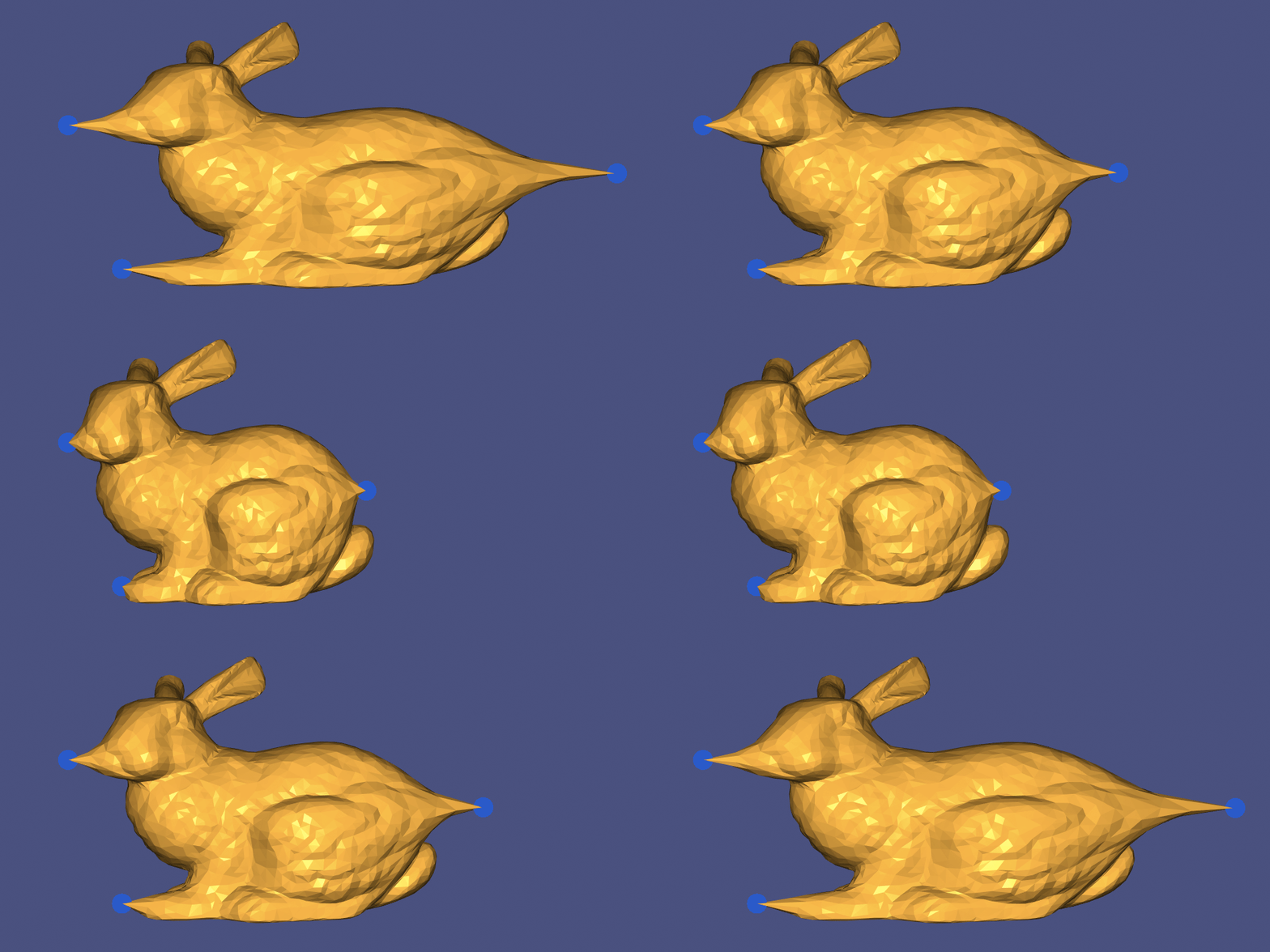
Biharmonic displacements work well for small deformations and deformations that
do not imply a large rotation. However, the Laplacian of the position function
This means that if the user transforms all of the handle locations by a rigid
transformation
As-rigid-as-possible
In the scenario where each handle
\[ \begin{align} ∫_Ω ‖ ∇ \x - ∇(\Rot \hat{\x} + \t) ‖² ;dA &= ∫_Ω ‖ ∇ \x - ∇(\Rot \hat{\x}) - ∇\t‖² ;dA \ &= ∫_Ω ‖ ∇ \x - \Rot ∇\hat{\x} ‖² ;dA, \end{align} \]
where the translation vector
We do not know the rotation
\[ ∫_Ω \left|∇\x - \left( \argmin_\Rot ∫_Ω ‖ ∇\x - \Rot ∇\hat{\x} ‖² ;dA \right)∇\hat{\x}\right|² ;dA. \]
If we treat
\[ \min_{\x,\Rot∈SO(3)} ∫_Ω \left|∇\x - \Rot ∇\hat{\x}\right|² ;dA. \]
Optimizing this energy will ensure global rotation invariance. To ensure
local rotation invariance, we can replace
For embedded solid shapes, we can take the rest shape given by
$\hat{\x}$ as the parameterization$Ω$ , so that$∇\hat{\x} = \I$ . This allows us to rewrite the as-rigid-as-possible energy as the square of the difference between the deformation gradient and the closest rotation:\[ ∫_Ω \left|∇\x - \Rot ∇\hat{\x}\right|² ;dA \ ∫_Ω \left|(∇\x + \I - \I) - \Rot \I \right|² ;dA \ ∫_Ω \left|(\I + ∇\x - ∇\hat{x}) - \Rot \right|² ;dA \ ∫_Ω \left|(\I + ∇\d) - \Rot \right|² ;dA \ ∫_Ω \left|\F - \Rot \right|² ;dA \ \]
This form provides a bridge between the as-rigid-as-possible energy common in geometry processing to corotated linear elasticity used in mechanics/physically-based simulation (made explicit in "A simple geometric model for elastic deformations" [Chao et al. 2010]). See Section 3.4 of "FEM Simulation of 3D Deformable Solids" [Sifakis 2012] for a graphics-mechanics perspective.
Discrete as-rigid-as-possible energy
For a triangle mesh with displacing vertices, the gradient of the embedding
function is constant inside each triangle. In this way we can write the raw
gradient energy above as a double sum over all half-edges
\[
½ ∫_Ω ‖ ∇ \x - ∇\hat{\x}‖² ;dA = ½ ∑\limits_{f ∈ F} ∑\limits_{ ij ∈ f} c_{ij} ‖
(\v_i-\v_j) - (\hat{\v}_i-\hat{\v}j)‖²,
\]
where $c{ij}$ is cotangent of the angle opposite half-edge
To inject localized best fit rotations, we will assign an unknown rotation
matrix
Where do rotations live?
We have assigned a rotation for each vertex: there are
$n$ rotation matrices as auxiliary degrees of freedom. This is in contrast to assigning rotations per face (as in "A Local/Global Approach to Mesh Parameterization" [Liu et al. 2008]). Per-face--or more generally per-element--rotations work well for codimension zero objects (triangle meshes in$\R²$ or tetrahedral meshes in$\R³$ ). But for triangle mesh surfaces in$\R³$ (i.e., codimension 1), per-face rotations would lead to "crumpling") because bending along edges would not be measured.
Optimization
The simplest method for optimizing the ARAP energy is by alternating between
- finding the optimal rotations
$\Rot_k$ assuming the vertex positions$\V$ are fixed, and - finding the optimal vertex positions
$\V$ assuming all rotations$\Rot_k$ are fixed.
Each rotation
Observing the discrete energy above we can see that the energy is quadratic in
\[ ⅙ \underbrace{∑\limits_{k=1}^n ∑\limits_{ ij ∈ F(k)} c_{ij} (\v_i-\v_j)^\transpose(\v_i-\v_j)}\text{quadratic} + ⅙ \underbrace{∑\limits{k=1}^n ∑\limits_{ ij ∈ F(k)} c_{ij} (\v_i-\v_j)^\transpose \Rot_k (\hat{\v}_i-\hat{\v}j)}\text{linear} \]
if we stack the rotation matrices
\[
\tr{ \V^\transpose \L \V } + \tr{ \V^\transpose \K \Rot },
\]
where
I'm so confused. What's in the
$\K$ matrix?Let's take it slow. The
$\K$ matrix is represents the bilinear form that combines unknown vertex positions and unknown rotations. We have identified above that we can write this in summation or matrix form: \[ ⅙ ∑\limits_{k=1}^n ∑\limits_{ ij ∈ F(k)} c_{ij} (\v_i-\v_j)^\transpose \Rot_k (\hat{\v}_i-\hat{\v}_j) = \tr{ \V^\transpose \K \Rot }, \] but how did we get here?Let's start with the summation form. The constants of this formula are the
$c_{ij}$ terms and the $(\hat{\v}_i-\hat{\v}j)$ terms. Since these always appear together, let us merge them into weighted edge difference vectors $c{ij} (\hat{\v}_i-\hat{\v}j) =: \hat{\e}{ij} ∈ \R³$:\[ ⅙ ∑\limits_{k=1}^n ∑\limits_{ ij ∈ F(k)} \underbrace{(\v_i-\v_j)^\transpose \Rot_k \hat{\e}{ij}}{∈\R}, \] the inner term in the summation is an inner product; that is, a scalar. Let's expose this by expanding the matrix-vector products of the inner-product: \[ ⅙ ∑\limits_{k=1}^n ∑\limits_{ ij ∈ F(k)} ∑\limits_{α=1}^3 ∑\limits_{β=1}^3 (v_i^α - v_j^α)R_k^{αβ}\hat{e}_{ij}^β. \]
If our mesh is stored as a vertex list and face list, it's not easy/efficient to loop over per-vertex rotations (outer sum) and then over all half-edges of incident faces (second sum). Instead, let's rearrange these sums to loop over all faces first, then the half-edges of that face, and then over all per-vertex rotations that involve this half-edge: \[ ⅙ ∑\limits_{f=1}^m ∑\limits_{ ij ∈ E(f)} \quad ∑\limits_{k | ij ∈F(k)} \quad ∑\limits_{α=1}^3 ∑\limits_{β=1}^3 (v_i^α - v_j^α)R_k^{αβ}\hat{e}_{ij}^β, \] where the third sum is over all rotations
$k$ such that the half-edge$ij$ belongs to the half-edges of the faces incident on the$k$ -th vertex:$k | ij ∈F(k)$ . Well, this means$k$ can either be$i$ or$j$ or the third vertex of the$f$ -th face.Now let's turn our attention back to the summand. The terms indexed by
$α$ never mix. That is, we never add/multiply$v_i^α$ ,$v_j^γ$ , and$R_k^{δβ}$ unless$α=γ=δ$ . This implies that we can write this summation in matrix form as: \[ \V₁^\transpose \K₁ \Rot₁ +
\V₂^\transpose \K₂ \Rot₂ +
\V₃^\transpose \K₃ \Rot₃, \] where$\V_α ∈ \R^n$ is$α$ -th column of$\V$ ,$\Rot_α ∈ \R^{3n}$ is the$α$ -th column of$\Rot$ and$\K₁,\K₂,\K₃ ∈ \R^{n × 3n}$ are sparse matrices.Further, the constant term
$\hat{e}^β_{ij}$ in the summation acts the same on$(v_i^α - v_j^α)R_k^{αβ}$ for any$α$ value. This implies that$\K₁=\K₂=\K₃$ , so we can reduce the matrix form to: \[ \tr{\V \K \Rot}. \]Finally, we can answer what is in each entry
$K_{vw}$ , where$v$ chooses the row and$w=3k+β$ chooses the column of$\K$ . Treating our nested summation as nested for-loops, we can increment entries in$\K$ \[ \begin{align} K_{i\ 3k+β} & \mathrel{+}= \hat{e}{ij}^β, \ K{j\ 3k+β} & \mathrel{+}= -\hat{e}_{ij}^β, \ \end{align} \] for each half-edge encountered.
Local step
Minimizing this energy with respect
\[
\tr{ \underbrace{\V^\transpose \K}_{\C^\transpose} \Rot },
\]
where
Global step
Minimizing the energy above with respect to
\[ \min_\V \tr{ \V^\transpose \L \V } + \tr{ \V^\transpose \B } \]
where
Implementation
In order to facilitate interactive deformation we would like our local and
global iterations to be computed as quickly as possible. Since the quadratic
form in the global step is the same regardless of the current rotations or
current handle positions, we can
prefactorize it (again,
as above). The matrix
Note: When constructing
$\K$ it's easiest to iterate over all half-edges in the mesh (by iterating over all faces and then each of the three edges). Each half-edge$ij$ contributes terms tying$\v_i,\v_j$ to each of the (three) rotations$\Rot_k$ that apply against their difference (see "Fast Automatic Skinning Transformations" [Jacobson et al. 2012]).
Still trouble in paradise
The as-rigid-as-possible deformation method for surfaces described above has a number of remaining problems:
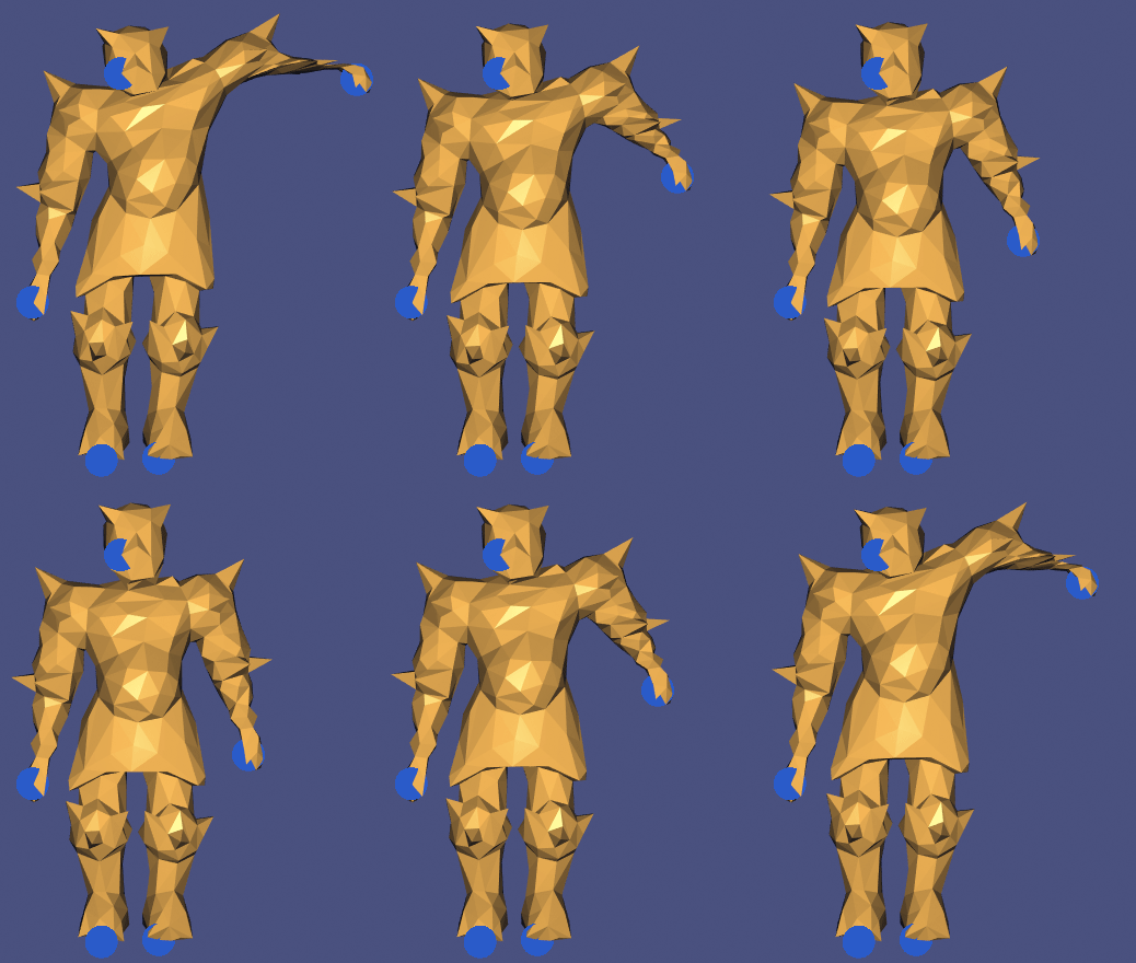
- like its gradient-based energy ancestor the deformation is not smooth at constraints;
- the energy punishes bending of the surface--which is good--but does so in a way that diminishes as the mesh becomes higher and higher resolution, in otherwords, the discrete energy is mesh-resolution dependent; and
- the energy is biased by the original combinatorics of the mesh (even in flat regions).
Tasks
Blacklist
igl::arapigl::arap_linear_blockigl::covariance_scatter_matrixigl::harmonic
Whitelist
igl::polar_svd3x3(or your previous assignment'sclosest_rotation)igl::min_quad_with_fixedigl::cotmatrix_entriesigl::cotmatrix(or your previous implementation)igl::massmatrix(or your previous implementation)
src/biharmonic_precompute.cpp
Precompute data needed to efficiently solve for a biharmonic deformation given
a mesh with vertices V and faces F and a list of selected vertices as
indices b into V. The output should be a prefacorized system using the
data struct employed by igl::min_quad_with_fixed.
src/biharmonic_solve.cpp
Given precomputation data and a list of handle displacements determine
displacements for all vertices in the mesh.
src/arap_precompute.cpp
Precompute data needed to efficiently conduct local-global iterations for an
arap deformation. This includes the data struct employed by
igl::min_quad_with_fixed to solve the global step" and constructing the
bilinear form K that mixes rotation degrees of freedom with unknown
positions for preparing the covariance matrices of the local step and the
linear term of the global step.
src/arap_single_iteration.cpp
Given precomputed data (data and K), handle positions bc and current
positions of all vertices U, conduct a single iteration of the local-global
solver for minimizing the as-rigid-as-possible energy. Output the positions
of all vertices of the mesh (by overwriting U).
