ddarmon/sfinsc-day3

Day 3 — Complex Network Visualization

Downloads and Setup

We will be using muxViz for this hands-on session. Download muxViz here by clicking on the "Download it from github" button.

Unzip the muxViz download and place the muxViz-master folder in your Documents folder.

If you are using a Mac, you will need to install XQuartz to interact with visualizations. Download XQuartz here.

For all platforms, muxViz requires the Java SE Development Kit (JDK) to run rJava in R. Download the JDK here. If you are running Windows, you will need to download either the 32-bit version (x86) or the 64-bit version (x64) depending on you computer. To determine the architecture of your machine, open Control Panel and browse to

Systems and Security > System

and look under "System type:" for the processor type.

Open RStudio. Navigate to the muxViz-master folder in the file browser, and click on the More button, and choose Set As Working Directory.

Now, from the RStudio Console, run

source('muxVizGUI.R')

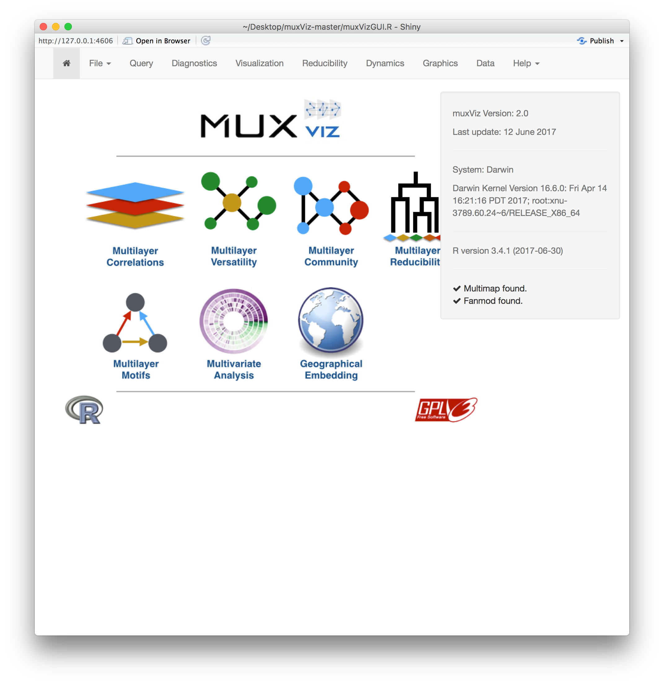
This script will install all of the R libraries required by muxViz. This may take a while. After all of the R libraries have been installed, the Shiny interface to R will open as a stand-alone browser window. You should see the following window:

Possible Bugs

Missing Packages

muxViz is designed for version 3.2 of R. Therefore, some of the packages may not load correctly with version 3.4 of R.

If you get the error

Error in library(ShinyDash) : there is no package called ‘ShinyDash’

run

require(devtools) install_github("ShinyDash", "trestletech")

in the Console to install ShinyDash.

If you get the error

Error in library(rCharts) : there is no package called ‘rCharts’

run

require(devtools) install_github('rCharts', 'ramnathv')

Java Error in Mac OS

If you are running Mac OS and run into a problem with rJava, run

sudo ln -f -s $(/usr/libexec/java_home)/jre/lib/server/libjvm.dylib /usr/local/lib

after you have installed Java 8 as above.

Multilayer Networks

As we learned earlier today, a multilayer network is a generalization of the monolayer representation we learned about on Wednesday that allows for nodes and edges to take on multiple roles. For example, in a social network, certain connections may be work-, family-, or friend-based, and treating all of those edges as the same

Manlio De Domenico, one of the creators of muxViz, curates a large collection of multilayer networks here.

Let's work through the muxViz demo put together by Manlio here.

Monolayer and Multilayer Analysis of an Online Social Network

User activity on social media (Twitter, Facebook, Instagram, etc.) is a rich source of data that can be readily handled by a network formalism. Relationships and interactions on social media sites can take many forms, and thus we should be certain to include the multifaceted nature of user-user interaction in constructing our networks. For this example, we will be working the data set from this paper, which explored interaction of 6918 users on Twitter over the 9 week period from April 25th to June 25th 2011. This time period is halfway through Twitter's history to-date. Twitter began as a microblogging platform in 2006 where messages were posted to the service through SMS. Now Twitter has over 300 million monthly active users. For a review of Twitter's history, check out this article by Wired.

Thus, this network has at least three types of directed links:

• An edge exists from User A to User B if User B follows User A.
• An edge exists from User A to User B if User A mentions User B.
• An edge exists from User A to User B if User B retweets User A.

The associated network files are in the data directory, and are named twitter_{following,mentions,retweets}.graphml and twitter_network_{following,mentions,retweets}.edges. Because the .edges files do not necessarily contain all of the nodes in the network, I have also included a twitter_network.nodes that lists the 6918 users.

Explore: Open the files in Sublime Text and investigate their structure. In the .edges files, what are the sources and targets in the following, mentions, and retweets files?

Monolayer Analysis of Twitter Networks

Using Gephi

A monolayer analysis would consider each of the network representations of the interactions between users in turn. For example, let's consider the followers network.

Explore: Load the mentions network into Gephi using the associated graphml file. How many nodes are in the network? How many edges?

As we have seen, Gephi initially loads the network without applying any sort of layout to the nodes. Let's apply a Layout to get a handle on the structure present in the network.

Explore: Apply some of the graph layouts to the followers network. Choose one that seems to highlight the meso-scale structure of the network.

Let's also compute some network statistics.

Explore: Compute the in- and out-degree of each node, and the degree distribution. For the representation we chose (an edge exists from User A to User B if User B follows User A), what does a large in-degree mean? What does a large out-degree mean?

Remember that you can change layout attributes like node size by using the Appearance panel.

Explore: Set the node sizes to scale according to the in-/out-degree.

Hint: To make the node degrees more obvious, you can turn off the edges by clicking the edge icon in the bottom left of the Graph panel (to the right of the T).

We can see a meso-scale structure in the following network: there appear to be groups of users who are more densely connected to other users in their group than to users in other groups. This is one kind of community structure. Gephi can attempt to find these communities through the Modularity routine in the Statistics panel, using the Louvain method for community detection.

Explore: Run the Modularity routine in the Statistics. Use the Appearance panel to color the nodes in the network according to their community membership. Does the coloring match how you would have expected the communities to turn out?

We have investigated some of the properties of the Twitter following network. But this is just a structural representation of the interaction between users: it only demonstrates who is following whom. The mentions and retweet networks will capture how the users actually interact. These interactions are guided by the following network: a user will only see a non-mention tweet of another user in their timeline if they are following that user, and will likely only see the tweet of a non-followed user when that tweet is retweeted by a user they do follow.

Let's investigate the other Twitter networks in Gephi.

Exercise: Investigate each of the following and retweets network, using some of the analyses above. In particular, you might investigate the general meso-scale structure, link density, in-/out-degrees, and community structure in the different networks.

Hint: When comparing various monolayer representations of the same network, it can be handy to use the Workspaces functionality of Gephi. When importing a new network, first create a new Workspace by selecting Workspace > New. You can also rename the Workspace (for example, to Following, Mentions, or Retweets) by selecting Workspace > Rename.

Hint: In the mentions and retweets networks, there will be 'orphan' users that did not / were not mentioned / retweeted. These nodes without any links may be hard to make out in the default view used in Gephi. Changing the Node size to 40 or larger will make these nodes stand out more.

Using igraph in R

As you may have noticed, Gephi can become sluggish as the density of the network (the number of edges out of all possible edges) increases. In this case, we can turn from Gephi to igraph in R, which can handle much larger networks since it does not need to render the network as we go.

Let's reproduce some of the analyses we did using Gephi in igraph, and perform some additional analyses.

Pointer: The R scripts I provided will assume that the network files are all in the data directory of the sfinsc-day3-master directory. Move the files in the shared Dropbox directory day3-data/data/for-gephi-network-files into the sfinsc-day3-master/data directory.

Explore: Run through the analysis in igraph-example-single.R line-by-line for the following, mentions, and retweet networks, and compare the results to those obtained using Gephi. To switch which edge type you consider, comment / uncomment the appropriate link.type lines.

One of the strengths of igraph relative to Gephi is the inclusion of many methods for investigating the meso-scale structure of a network. igraph has many more community detection algorithms beyond Louvain. Let's use the 'fast-greedy algorithm' (the common name for the algorithm presented in this paper by Aaron Clauset, Mark Newman, and Cristopher Moore) to further investigate the community structure in the network.

One way to quantify how similar the detected communities are in the following, mentions, and retweets networks is the compute the variation of information between the community partitions for two types of networks. The variation of information, or VI, is a metric on the space of clusterings, and thus is small for similar clustering and large for dissimilar clustering. It can be bounded between 0 and 2 log |V|, where |V| is the number of vertices in the network. Thus, we can get a normalized metric between 0 and 1 by dividing the variation of information by 2 log |V|.

The compare function in igraph will compute the variation of information between two partitions of the same node set.

Explore: Use igraph-example-compare.R to compute the variation of information between each pair of networks after determining their communities.

Multilayer Analysis of Twitter Networks using muxViz

Rather than consider each of the following, mentions, and retweets networks separately as monolayers, we can consider a multilayer representation of the network where the nodes are the users and the edges are colored based on the type of relationship: a following type, a retweet type, or a mention type.

As you might expect, the analysis of a multilayer network generally takes more computing than the analysis of a multilayer network: the analysis of three layers is at least as hard as the analysis of each layer in isolation, and usually harder. Because of this, for the sake of run time, we will focus on the multilayer network constructed using the retweets and mentions monolayers.

Pointer: Be sure to put the twitter directory into muxViz-master/data before trying to import into muxViz.

Explore: Investigate the *_config.txt, *_layout.txt, and *_layout.txt files in the muxViz-master/data/twitter folder. Use Sublime Text to open these files.

Explore: Open muxViz in RStudio. Select the twitter_mentions_config.txt config file, and load the monolayer into muxViz.

Explore: Experiment with using muxViz to analyze the network.

Explore: Create a *_config.txt file for the retweets network.

Explore: Load the retweets monolayer network into muxViz. Experiment with using muxViz to analyze the network.

Explore: Select the twitter_small-multiplex_config.txt config file (which includes only the retweets and mentions monolayers), and load the two monolayers into muxViz as a multilayer network.

Explore: Experiment with using muxViz to analyze the multilayer network.