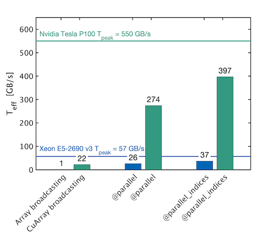
ParallelStencil empowers domain scientists to write architecture-agnostic high-level code for parallel high-performance stencil computations on GPUs and CPUs. Performance similar to CUDA C can be achieved, which is typically a large improvement over the performance reached when using only CUDA.jl Array programming. For example, a 2-D shallow ice solver presented at JuliaCon 2020 [1] achieved a nearly 20 times better performance than a corresponding CUDA.jl Array programming implementation; in absolute terms, it reached 70% of the theoretical upper performance bound of the used Nvidia P100 GPU, as defined by the effective throughput metric, T_eff (note that T_eff is very different from common throughput metrics, see section Performance metric). The GPU performance of the solver is reported in green, the CPU performance in blue:
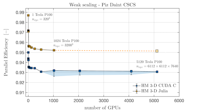
ParallelStencil relies on the native kernel programming capabilities of CUDA.jl and on Base.Threads for high-performance computations on GPUs and CPUs, respectively. It is seamlessly interoperable with ImplicitGlobalGrid.jl, which renders the distributed parallelization of stencil-based GPU and CPU applications on a regular staggered grid almost trivial and enables close to ideal weak scaling of real-world applications on thousands of GPUs [1, 2, 3, 4]. Moreover, ParallelStencil enables hiding communication behind computation with a simple macro call and without any particular restrictions on the package used for communication. ParallelStencil has been designed in conjunction with ImplicitGlobalGrid.jl for simplest possible usage by domain-scientists, rendering fast and interactive development of massively scalable high performance multi-GPU applications readily accessible to them. Furthermore, we have developed a self-contained approach for "Solving Nonlinear Multi-Physics on GPU Supercomputers with Julia" relying on ParallelStencil and ImplicitGlobalGrid.jl [1]. ParallelStencil's feature to hide communication behind computation was showcased when a close to ideal weak scaling was demonstrated for a 3-D poro-hydro-mechanical real-world application on up to 1024 GPUs on the Piz Daint Supercomputer [1]:
A particularity of ParallelStencil is that it enables writing a single high-level Julia code that can be deployed both on a CPU or a GPU. In conjuction with ImplicitGlobalGrid.jl the same Julia code can even run on a single CPU thread or on thousands of GPUs/CPUs.
- Parallelization with one macro call
- Stencil computations with math-close notation
- 50-lines example deployable on GPU and CPU
- 50-lines multi-XPU example
- Seamless interoperability with communication packages and hiding communication
- Support for architecture-agnostic low level kernel programming
- Module documentation callable from the Julia REPL / IJulia
- Concise single/multi-XPU miniapps
- Dependencies
- Installation
- Questions, comments and discussions
- References
A simple call to @parallel is enough to parallelize a function and to launch it. The package used underneath for parallelization is defined in a call to @init_parallel_stencil beforehand. Supported are CUDA.jl for running on GPU and Base.Threads for CPU. The following example outlines how to run parallel computations on a GPU using the native kernel programming capabilities of CUDA.jl underneath (omitted lines are represented with #(...), omitted arguments with ...):
#(...)
@init_parallel_stencil(CUDA,...);
#(...)
@parallel function diffusion3D_step!(...)
    #(...)
end
#(...)
@parallel diffusion3D_step!(...)
Note that arrays are automatically allocated on the hardware chosen for the computations (GPU or CPU) when using the provided allocation macros:
@zeros@ones@rand
ParallelStencil provides submodules for computing finite differences in 1-D, 2-D and 3-D with a math-close notation (FiniteDifferences1D, FiniteDifferences2D and FiniteDifferences3D). Custom macros to extend the finite differences submodules or for other stencil-based numerical methods can be readily plugged in. The following example shows a complete function for computing a time step of a 3-D heat diffusion solver using FiniteDifferences3D.
#(...)
using ParallelStencil.FiniteDifferences3D
#(...)
@parallel function diffusion3D_step!(T2, T, Ci, lam, dt, dx, dy, dz)
    @inn(T2) = @inn(T) + dt*(lam*@inn(Ci)*(@d2_xi(T)/dx^2 + @d2_yi(T)/dy^2 + @d2_zi(T)/dz^2));
    return
end
The macros used in this example are described in the Module documentation callable from the Julia REPL / IJulia:
julia> using ParallelStencil.FiniteDifferences3D
julia>?
help?> @inn
  @inn(A): Select the inner elements of A. Corresponds to A[2:end-1,2:end-1,2:end-1].

help?> @d2_xi
  @d2_xi(A): Compute the 2nd order differences between adjacent elements of A along the along dimension x and select the inner elements of A in the remaining dimensions. Corresponds to @inn_yz(@d2_xa(A)).
Note that@d2_yi and @d2_zi perform the analogue operations as @d2_xi along the dimension y and z, respectively.
Type ?FiniteDifferences3D in the Julia REPL to explore all provided macros.
This concise 3-D heat diffusion solver uses ParallelStencil and a a simple boolean USE_GPU defines whether it runs on GPU or CPU (the environment variable JULIA_NUM_THREADS defines how many cores are used in the latter case):
const USE_GPU = true
using ParallelStencil
using ParallelStencil.FiniteDifferences3D
@static if USE_GPU
    @init_parallel_stencil(CUDA, Float64, 3);
else
    @init_parallel_stencil(Threads, Float64, 3);
end

@parallel function diffusion3D_step!(T2, T, Ci, lam, dt, dx, dy, dz)
    @inn(T2) = @inn(T) + dt*(lam*@inn(Ci)*(@d2_xi(T)/dx^2 + @d2_yi(T)/dy^2 + @d2_zi(T)/dz^2));
    return
end

function diffusion3D()
# Physics
lam        = 1.0;                                        # Thermal conductivity
cp_min     = 1.0;                                        # Minimal heat capacity
lx, ly, lz = 10.0, 10.0, 10.0;                           # Length of domain in dimensions x, y and z.

# Numerics
nx, ny, nz = 256, 256, 256;                              # Number of gridpoints dimensions x, y and z.
nt         = 100;                                        # Number of time steps
dx         = lx/(nx-1);                                  # Space step in x-dimension
dy         = ly/(ny-1);                                  # Space step in y-dimension
dz         = lz/(nz-1);                                  # Space step in z-dimension

# Array initializations
T   = @zeros(nx, ny, nz);
T2  = @zeros(nx, ny, nz);
Ci  = @zeros(nx, ny, nz);

# Initial conditions (heat capacity and temperature with two Gaussian anomalies each)
Ci .= 1.0./( cp_min .+ Data.Array([5*exp(-(((ix-1)*dx-lx/1.5))^2-(((iy-1)*dy-ly/2))^2-(((iz-1)*dz-lz/1.5))^2) +
                                   5*exp(-(((ix-1)*dx-lx/3.0))^2-(((iy-1)*dy-ly/2))^2-(((iz-1)*dz-lz/1.5))^2) for ix=1:size(T,1), iy=1:size(T,2), iz=1:size(T,3)]) )
T  .= Data.Array([100*exp(-(((ix-1)*dx-lx/2)/2)^2-(((iy-1)*dy-ly/2)/2)^2-(((iz-1)*dz-lz/3.0)/2)^2) +
                   50*exp(-(((ix-1)*dx-lx/2)/2)^2-(((iy-1)*dy-ly/2)/2)^2-(((iz-1)*dz-lz/1.5)/2)^2) for ix=1:size(T,1), iy=1:size(T,2), iz=1:size(T,3)])
T2 .= T;                                                 # Assign also T2 to get correct boundary conditions.

# Time loop
dt = min(dx^2,dy^2,dz^2)*cp_min/lam/8.1;                 # Time step for the 3D Heat diffusion
for it = 1:nt
    @parallel diffusion3D_step!(T2, T, Ci, lam, dt, dx, dy, dz);
    T, T2 = T2, T;
end

end

diffusion3D()
The corresponding file can be found here.
This concise multi-XPU 3-D heat diffusion solver uses ParallelStencil in conjunction with ImplicitGlobalGrid.jl and can be readily deployed on on a single CPU thread or on thousands of GPUs/CPUs. Again, a simple boolean USE_GPU defines whether it runs on GPU(s) or CPU(s) (JULIA_NUM_THREADS defines how many cores are used in the latter case). The solver can be run with any number of processes. ImplicitGlobalGrid.jl creates automatically an implicit global computational grid based on the number of processes the solver is run with (and based on the process topology, which can be explicitly chosen by the user or automatically determined). Please refer to the documentation of ImplicitGlobalGrid.jl for more information.
const USE_GPU = true
using ImplicitGlobalGrid
import MPI
using ParallelStencil
using ParallelStencil.FiniteDifferences3D
@static if USE_GPU
    @init_parallel_stencil(CUDA, Float64, 3);
else
    @init_parallel_stencil(Threads, Float64, 3);
end

@parallel function diffusion3D_step!(T2, T, Ci, lam, dt, dx, dy, dz)
    @inn(T2) = @inn(T) + dt*(lam*@inn(Ci)*(@d2_xi(T)/dx^2 + @d2_yi(T)/dy^2 + @d2_zi(T)/dz^2));
    return
end

function diffusion3D()
# Physics
lam        = 1.0;                                        # Thermal conductivity
cp_min     = 1.0;                                        # Minimal heat capacity
lx, ly, lz = 10.0, 10.0, 10.0;                           # Length of domain in dimensions x, y and z.

# Numerics
nx, ny, nz = 256, 256, 256;                              # Number of gridpoints dimensions x, y and z.
nt         = 100;                                        # Number of time steps
init_global_grid(nx, ny, nz);
dx         = lx/(nx_g()-1);                              # Space step in x-dimension
dy         = ly/(ny_g()-1);                              # Space step in y-dimension
dz         = lz/(nz_g()-1);                              # Space step in z-dimension

# Array initializations
T   = @zeros(nx, ny, nz);
T2  = @zeros(nx, ny, nz);
Ci  = @zeros(nx, ny, nz);

# Initial conditions (heat capacity and temperature with two Gaussian anomalies each)
Ci .= 1.0./( cp_min .+ Data.Array([5*exp(-((x_g(ix,dx,Ci)-lx/1.5))^2-((y_g(iy,dy,Ci)-ly/2))^2-((z_g(iz,dz,Ci)-lz/1.5))^2) +
                                   5*exp(-((x_g(ix,dx,Ci)-lx/3.0))^2-((y_g(iy,dy,Ci)-ly/2))^2-((z_g(iz,dz,Ci)-lz/1.5))^2) for ix=1:size(T,1), iy=1:size(T,2), iz=1:size(T,3)]) )
T  .= Data.Array([100*exp(-((x_g(ix,dx,T)-lx/2)/2)^2-((y_g(iy,dy,T)-ly/2)/2)^2-((z_g(iz,dz,T)-lz/3.0)/2)^2) +
                   50*exp(-((x_g(ix,dx,T)-lx/2)/2)^2-((y_g(iy,dy,T)-ly/2)/2)^2-((z_g(iz,dz,T)-lz/1.5)/2)^2) for ix=1:size(T,1), iy=1:size(T,2), iz=1:size(T,3)])
T2 .= T;                                                 # Assign also T2 to get correct boundary conditions.

# Time loop
dt = min(dx^2,dy^2,dz^2)*cp_min/lam/8.1;                 # Time step for the 3D Heat diffusion
for it = 1:nt
    @parallel diffusion3D_step!(T2, T, Ci, lam, dt, dx, dy, dz);
    update_halo!(T2);
    T, T2 = T2, T;
end

finalize_global_grid();
end

diffusion3D()
The corresponding file can be found here.
Thanks to ImplicitGlobalGrid.jl, only a few function calls had to be added in order to turn the previous single GPU/CPU solver into a multi-XPU solver (omitted unmodified lines are represented with #(...)):
#(...)
using ImplicitGlobalGrid
#(...)
function diffusion3D()
# Physics
#(...)
# Numerics
#(...)
init_global_grid(nx, ny, nz);
dx  = lx/(nx_g()-1);                                     # Space step in x-dimension
dy  = ly/(ny_g()-1);                                     # Space step in y-dimension
dz  = lz/(nz_g()-1);                                     # Space step in z-dimension

# Array initializations
#(...)

# Initial conditions (heat capacity and temperature with two Gaussian anomalies each)
Ci .= 1.0./( cp_min .+ Data.Array([5*exp(-((x_g(ix,dx,Ci)-lx/1.5))^2-((y_g(iy,dy,Ci)-ly/2))^2-((z_g(iz,dz,Ci)-lz/1.5))^2) +
                                   5*exp(-((x_g(ix,dx,Ci)-lx/3.0))^2-((y_g(iy,dy,Ci)-ly/2))^2-((z_g(iz,dz,Ci)-lz/1.5))^2) for ix=1:size(T,1), iy=1:size(T,2), iz=1:size(T,3)]) )
T  .= Data.Array([100*exp(-((x_g(ix,dx,T)-lx/2)/2)^2-((y_g(iy,dy,T)-ly/2)/2)^2-((z_g(iz,dz,T)-lz/3.0)/2)^2) +
                   50*exp(-((x_g(ix,dx,T)-lx/2)/2)^2-((y_g(iy,dy,T)-ly/2)/2)^2-((z_g(iz,dz,T)-lz/1.5)/2)^2) for ix=1:size(T,1), iy=1:size(T,2), iz=1:size(T,3)])

# Time loop
#(...)
for it = 1:nt
    #(...)
    update_halo!(T2);
    #(...)
end

finalize_global_grid();
end

diffusion3D()
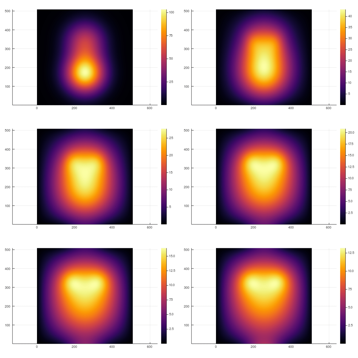
Here is the resulting movie when running the application on 8 GPUs, solving 3-D heat diffusion with heterogeneous heat capacity (two Gaussian anomalies) on a global computational grid of size 510x510x510 grid points. It shows the x-z-dimension plane in the middle of the dimension y:
The corresponding file can be found here.
The previous multi-XPU example shows that ParallelStencil is seamlessly interoperable with ImplicitGlobalGrid.jl. The same is a priori true for any communication package that allows to explicitly decide when the required communication occurs; an example is MPI.jl (besides, MPI.jl is also seamlessly interoperable with ImplicitGlobalGrid.jl and can extend its functionality).
Moreover, ParallelStencil enables hiding communication behind computation with as simple call to @hide_communication. In the following example, the communication performed by update_halo! (from the package ImplicitGlobalGrid.jl) is hidden behind the computations done with by @parallel diffusion3D_step!:
@hide_communication (16, 2, 2) begin
    @parallel diffusion3D_step!(T2, Te Ci, lam, dt, dx, dy, dz);
    update_halo!(T2);
end
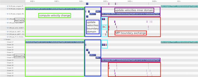
This enables close to ideal weak scaling of real-world applications on thousands of GPUs/CPUs [1, 2]. Type ?@hide_communication in the Julia REPL to obtain an explanation of the arguments. Profiling a 3-D viscous Stokes flow application using the Nvidia visual profiler (nvvp) graphically exemplifies how the update velocities kernel is split up in boundary and inner domain computations and how the latter overlap with point-to-point MPI communication for halo exchange:
High-level stencil computations with math-close notation can be completed with index-based programming using the macro @parallel_indices. For example, the following kernel enables setting Neumann boundary conditions in dimension y (∂A/∂y = 0) when using finite differences in 3-D:
@parallel_indices (ix,iz) function bc_y!(A)
    A[ix,   1, iz] = A[ix,     2, iz]
    A[ix, end, iz] = A[ix, end-1, iz]
    return
end
It can be launched as follows:
@parallel (1:size(A,1), 1:size(A,3)) bc_y!(A)Furthermore, a set of architecture-agnostic low level kernel language constructs is supported in these @parallel_indices kernels (see in Module documentation callable from the Julia REPL / IJulia). They enable, e.g., explicit usage of shared memory (see this 2-D heat diffusion example).
The module documentation can be called from the Julia REPL or in IJulia:
julia> using ParallelStencil
julia>?
help?> ParallelStencil
search: ParallelStencil @init_parallel_stencil

  Module ParallelStencil

  Enables domain scientists to write high-level code for parallel high-performance stencil computations that can be deployed on both GPUs and CPUs.

  General overview and examples
  ≡≡≡≡≡≡≡≡≡≡≡≡≡≡≡≡≡≡≡≡≡≡≡≡≡≡≡≡≡≡≡

  https://github.com/omlins/ParallelStencil.jl

  Primary macros
  ≡≡≡≡≡≡≡≡≡≡≡≡≡≡≡≡

    •  @init_parallel_stencil

    •  @parallel

    •  @hide_communication

    •  @zeros

    •  @ones

    •  @rand

  │ Advanced
  │
  │    •  @parallel_indices
  │
  │    •  @parallel_async
  │
  │    •  @synchronize

  Macros available for @parallel_indices kernels
  ≡≡≡≡≡≡≡≡≡≡≡≡≡≡≡≡≡≡≡≡≡≡≡≡≡≡≡≡≡≡≡≡≡≡≡≡≡≡≡≡≡≡≡≡≡≡≡≡

    •  @ps_show

    •  @ps_println

  │ Advanced
  │
  │    •  @gridDim
  │
  │    •  @blockIdx
  │
  │    •  @blockDim
  │
  │    •  @threadIdx
  │
  │    •  @sync_threads
  │
  │    •  @sharedMem

  Submodules
  ≡≡≡≡≡≡≡≡≡≡≡≡

    •  ParallelStencil.FiniteDifferences1D

    •  ParallelStencil.FiniteDifferences2D

    •  ParallelStencil.FiniteDifferences3D

  Modules generated in caller
  ≡≡≡≡≡≡≡≡≡≡≡≡≡≡≡≡≡≡≡≡≡≡≡≡≡≡≡≡≡

    •  Data

To see a description of a macro or module type ?<macroname> (including the @) or ?<modulename>, respectively.The miniapps regroup a collection of various 2-D and 3-D codes that leverage ParallelStencil to implement architecture-agnostic high-level code for parallel high-performance stencil computations on GPUs and CPUs. The miniapps target various challenging domain science case studies where multi-physics coupling and important nonlinearities challenge existing solving strategies. In most cases, second order pseudo-transient relaxation delivers implicit solutions of the differential equations. Some miniapps feature a multi-XPU version, which combines the capabilities of ParallelStencil and ImplicitGlobalGrid.jl in order to enable multi-GPU and multi-CPU executions, unleashing Julia-at-scale.
Many-core processors as GPUs are throughput-oriented systems that use their massive parallelism to hide latency. On the scientific application side, most algorithms require only a few operations or flops compared to the amount of numbers or bytes accessed from main memory, and thus are significantly memory bound. The Flop/s metric is no longer the most adequate for reporting the application performance of many modern applications. This status motivated us to develop a memory throughput-based performance evaluation metric, T_eff, to evaluate the performance of iterative stencil-based solvers [1].
The effective memory access, A_eff [GB], is the the sum of twice the memory footprint of the unknown fields, D_u, (fields that depend on their own history and that need to be updated every iteration) and the known fields, D_k, that do not change every iteration. The effective memory access divided by the execution time per iteration, t_it [sec], defines the effective memory throughput, T_eff [GB/s].
The upper bound of T_eff is T_peak as measured e.g. by the [7] for CPUs or a GPU analogue. Defining the T_eff metric, we assume that 1) we evaluate an iterative stencil-based solver, 2) the problem size is much larger than the cache sizes and 3) the usage of time blocking is not feasible or advantageous (which is a reasonable assumption for real-world applications). An important concept is not to include fields within the effective memory access that do not depend on their own history (e.g. fluxes); such fields can be re-computed on the fly or stored on-chip. Defining a theoretical upper bound for T_eff that is closer to the real upper bound is work in progress.
Using simple array broadcasting capabilities both with GPU and CPU arrays within Julia does not enable close to optimal performance; ParallelStencil.jl permits to overcome this limitation (see top figure) at similar ease of programming.
- Thermo-mechanical convection 2-D app
- Viscous Stokes 2-D app
- Viscous Stokes 3-D app
- Acoustic wave 2-D app
- Acoustic wave 3-D app
- Scalar porosity waves 2-D app
- Hydro-mechanical porosity waves 2-D app
- More to come, stay tuned...
All miniapp codes follow a similar structure and permit serial and threaded CPU as well as Nvidia GPU execution. The first line of each miniapp code permits to enable the CUDA GPU backend upon setting the USE_GPU flag to true.
All the miniapps can be interactively executed within the Julia REPL (this includes the multi-XPU versions when using a single CPU or GPU). Note that for optimal performance the miniapp script of interest <miniapp_code> should be launched from the shell using the project's dependencies --project, disabling array bound checking --check-bounds=no, and using optimization level 3 -O3.
$ julia --project --check-bounds=no -O3 <miniapp_code>.jlNote: refer to the documentation of your Supercomputing Centre for instructions to run Julia at scale. Instructions for running on the Piz Daint GPU supercomputer at the Swiss National Supercomputing Centre can be found here and for running on the octopus GPU supercomputer at the Swiss Geocomputing Centre can be found here.
This thermal convection example in 2-D combines a viscous Stokes flow to advection-diffusion of heat including a temperature-dependent shear viscosity. The miniapp resolves thermal convection cells (e.g. Earth's mantle convection and plumes):
The gif depicts non-dimensional temperature field as evolving into convection cells and plumes. Results are obtained by running the miniapp ThermalConvection2D.jl.
app: Stokes2D.jl
The viscous Stokes flow example solves the incompressible Stokes equations with linear shear rheology in 2-D. The model configuration represents a buoyant inclusion within a less buoyant matrix:
The figure depicts - Upper panels: the dynamical pressure field, the vertical Vy velocity. Lower pannels: the log10 of the vertical momentum balance residual Ry and the log10 of the error norm evolution as function of pseudo-transient iterations. Results are obtained by running the miniapp Stokes2D.jl.
apps: Stokes3D.jl, Stokes3D_multixpu.jl
The viscous Stokes flow example solves the incompressible Stokes equations with linear shear rheology in 3-D. The model configuration represents a buoyant spherical inclusion within a less buoyant matrix:
The figure depicts vertically sliced cross-sections of - Upper panels: the dynamical pressure field, the vertical Vz velocity. Lower panels: the log10 of the vertical momentum balance residual Rz and the log10 of the error norm evolution as function of pseudo-transient iterations. The numerical resolution is 252x252x252 grid points in 3-D on 8 GPUs (i.e. a local domain size of 127x127x127 per GPU). The Stokes3D.jl and Stokes3D_multixpu.jl are single- and multi-XPU implementations, respectively. The multi-XPU implementation demonstrates ParallelStencil's capabilities to hide computations behind communication, which is performed with ImplicitGlobalGrid.jl in this case. Results are obtained by running the multi-XPU miniapp Stokes3D_multixpu.jl on 8 Nvidia Titan Xm GPUs distributed across two physically distinct compute nodes.
This multi-XPU application permits to leverage distributed memory parallelisation to enable large-scale 3-D calculations.
app: acoustic2D.jl
The acoustic wave example solves acoustic waves in 2-D using the split velocity-pressure formulation:
The animation depicts the dynamical pressure field evolution as function of explicit time steps. Results are obtained by running the miniapp acoustic2D.jl.
The acoustic wave examples solves acoustic waves in 3-D using the split velocity-pressure formulation:
The animation depicts the y-slice of the dynamical pressure field evolution as function of explicit time steps. The achieved numerical resolution is 1020x1020x1020 grid points in 3-D on 8 GPUs (i.e. a local domain size of 511x511x511 per GPU). The acoustic3D.jl and acoustic3D_multixpu.jl are single- and multi-XPU implementation, respectively. The multi-XPU implementation demonstrates ParallelStencil's capabilities to hide computations behind communication, which is performed with ImplicitGlobalGrid.jl in this case. Results are obtained by running the multi-XPU miniapp acoustic3D_multixpu.jl on 8 Nvidia Titan Xm GPUs distributed across two physically distinct compute nodes.
This multi-XPU application permits to leverage distributed memory parallelisation to enable large-scale 3-D calculations.
The scalar porosity waves example solves the scalar solitary wave equations in 2-D assuming total pressure to be lithostatic, thus eliminating the need to solve for the total pressure explicitly:
The animation depicts the normalised porosity and effective pressure fields evolution as function of explicit time steps. Top row: compaction and decompaction rheology are identical, resulting in circular solitary waves rearranging into solitons of characteristic size. Bottom row: decompaction occurs at much faster rate compared to compaction, resulting in chimney-shaped features.
app: HydroMech2D.jl
The hydro-mechanical porosity wave example resolves solitary waves in 2-D owing to hydro-mechanical coupling, removing the lithostatic pressure assumption. The total and fluid pressure are explicitly computed from nonlinear Stokes and Darcy flow solvers, respectively [8]:
The animation depicts the formation of fluid escape pipes in two-phase media, owing to decompaction weakening running the miniapp HydroMech2D.jl. Top row: evolution of the porosity distribution and effective pressure. Bottom row: Darcy flux (relative fluid to solid motion) and solid (porous matrix) deformation.
ParallelStencil relies on the Julia CUDA package (CUDA.jl [5, 6]), MacroTools.jl and StaticArrays.jl.
ParallelStencil may be installed directly with the Julia package manager from the REPL:
julia>]
  pkg> add ParallelStencil
pkg> test ParallelStencilTo discuss technical issues, please post on Julia Discourse in the GPU topic or the Julia at Scale topic or in the #gpu or #distributed channels on the Julia Slack (to join, visit https://julialang.org/slack/).
To discuss numerical/domain-science issues, please post on Julia Discourse in the Numerics topic or the Modelling & Simulations topic or whichever other topic fits best your issue.


