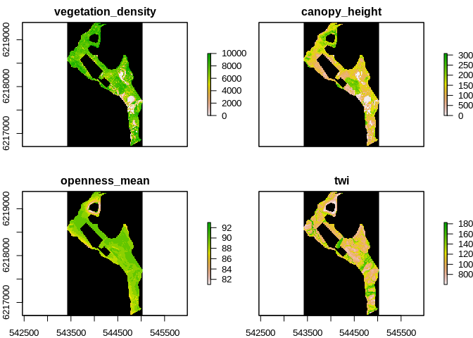
In order to include Vegetation complexity and wetness in the startification the following layers were used:
- vegetation height (“O:/Nat_Ecoinformatics-tmp/au634851/dk_lidar_backup_2021-06-28/canopy_height”)
- vegetation density (“O:/Nat_Ecoinformatics-tmp/au634851/dk_lidar_backup_2021-06-28/vegetation_density”)
- vegetation openness ("“O:/Nat_Ecoinformatics-tmp/au634851/dk_lidar_backup_2021-06-28/openness_mean”)
- TWI ("“O:/Nat_Ecoinformatics-tmp/au634851/dk_lidar_backup_2021-06-28/twi”)
Which resulted in this stack
The raster package was used for layer processing, sf for managing
shapefiles and the package GeoStratR was used for the stratification
of the site,
The preparation of rasters was made in the ‘Prepare_rasters.r’ in order to get all the rasters in the same resolution and crs
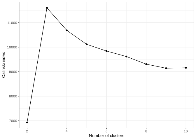
The Stratify function from GeoSratR was used in order to test the best
stratification from 2 to 10 groups, with the following results
In the graph bellow we can see that the number of classes that best captures the variablity is 3 as seen in the following graph
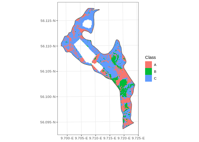
The Resulting raster of classes is the following:
Which leads to the following number of cells per class:
| Class | n |
|---|---|
| A | 3122 |
| B | 1382 |
| C | 5848 |
First we will generate 4 experimental plot groups at each class,
consisting of a fenced 15 by 15 meter point and and accompaning
monitoring plot. In order to do that we will generate 4 random points
with at least 40 meters from each other and from the border using the
Random_Stratified_Min_Dist function from the GeoStratR package:
#set seed for reproducibility


set.seed(2021)

Experimental <- Random_Stratified_Min_Dist(ClassRaster = FinalStack,
                           MinDist = 20,
                           n = 10,
                           n_to_test = 700)
##
## A B C
## 10 10 10
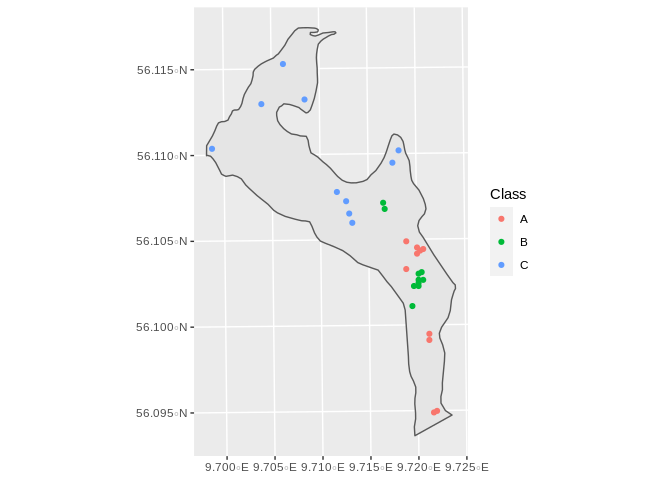
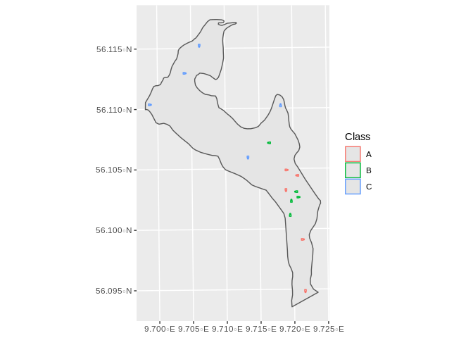
Which can be seen here:
## NULL
The sampling points are available in the Sampling folder
## Warning in dir.create("Sampling"): 'Sampling' already exists
Ranked plots
## NULL
