Dealing with Spatial Autocorrelation in a Gamma GLMM

Problem Overview

I am working with a dataset that examines plant growth in relation to various factors, including sea ice extent (SeaIce) at 14 different sampling sites. To analyze the data, I am using a Gamma Generalized Linear Mixed Model (GLMM) with a log-link function. However, I am concerned about spatial autocorrelation in the model’s residuals and I am unsure about the best approach to address this issue.

To solve this, I am utilizing the DHARMa package along with lme4 for model fitting.

library(DHARMa)
library(lme4)
library(MASS)
library(gstat)
library(dplyr)
library(sf)
library(sp)

You can find the dataset for this model in this GitHub repository.

FinalDataset <- read.csv("https://raw.githubusercontent.com/derek-corcoran-barrios/SeaIceQuestion/master/FinalDataset.csv")

Current Model Structure

Response Variable

Growth: Represents the annual growth increment of each individual plant.

Predictors

SeaIce.s: Sea ice extent per year per site, a primary predictor of interest (scaled).
age: Age of each individual plant for each measured year, included as an interaction with SeaIce.s due to a biological relationship between plant age and growth.

Random Effects

Site: A factor representing the 14 sampling sites with varying distances between them. I include a random slope (SeaIce.s | Site) to account for different slopes in the growth-sea ice relationship per site.
year: The study covers the years from 1983 to 2015 and is included as a random effect (1 | year).
Individual: A factor representing each individual plant measured.

Model

fullmod <- glmer(Growth ~ SeaIce.s * age + (SeaIce.s | Site) + (1 | year) + (1 | Individual), data = FinalDataset, family = Gamma(link = "log"), control = glmerControl(optimizer = "bobyqa", optCtrl = list(maxfun = 2e5)))

Primary Concern

My main concern is how to properly account for spatial autocorrelation within this model. I can see that there is a problem when I use this code in dHARMA.

res2_null <- simulateResiduals(fullmod)
res3_null <- recalculateResiduals(res2_null, group = FinalDataset$Site)
locs_null <- FinalDataset %>% group_by(Site) %>% summarise(across(c(Latitude, Longitude), mean))
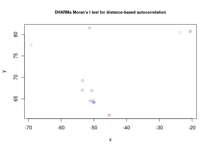
testSpatialAutocorrelation(res3_null, x = locs_null$Longitude, y = locs_null$Latitude)

## 
##  DHARMa Moran's I test for distance-based autocorrelation
## 
## data:  res3_null
## observed = 0.343448, expected = -0.076923, sd = 0.150983, p-value =
## 0.005365
## alternative hypothesis: Distance-based autocorrelation

As you can see by this result, there is a high spatial autocorrelation.

Some things I have tried:

Attempted Solution 1

One of the solutions I’ve attempted following this question to include latitude and longitude as fixed effects. However, when I test for spatial autocorrelation using testSpatialAutocorrelation() in the DHARMa package, I still get a significant Moran’s I with the model that includes latitude and longitude.

LonLatmod <- glmer(Growth ~ SeaIce.s * age + Latitude + Longitude + (SeaIce.s | Site) + (1 | year) + (1 | Individual), data = FinalDataset, family = Gamma(link = "log"), control = glmerControl(optimizer = "bobyqa", optCtrl = list(maxfun = 2e5)))

res <-  simulateResiduals(LonLatmod)
res2 <- recalculateResiduals(res, group = FinalDataset$Site)
locs_latlon <- FinalDataset %>% group_by(Site) %>% summarise(across(c(Latitude, Longitude), mean))
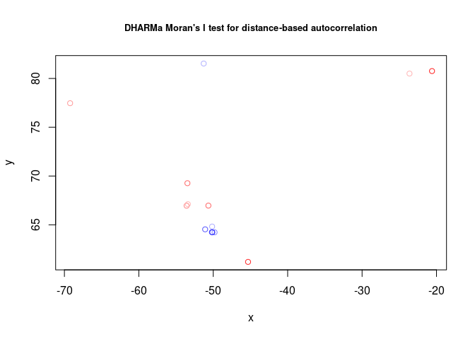
testSpatialAutocorrelation(res2, x =  locs_latlon$Longitude, y = locs_latlon$Latitude)

## 
##  DHARMa Moran's I test for distance-based autocorrelation
## 
## data:  res2
## observed = 0.382948, expected = -0.076923, sd = 0.150649, p-value =
## 0.002269
## alternative hypothesis: Distance-based autocorrelation

Attempted Solution 2

I also tried using glmmPQL() in the MASS package. But I have not been able to get this to work either, due to various errors, even without adding the correlation structure. Example below:

formula_glmmPQL <- as.formula("Growth ~ SeaIce.s * age")
model_glmmPQL <- glmmPQL(formula_glmmPQL,
                         random = list(~ SeaIce.s|Site, 
                                      ~ 1|year, 
                                      ~1| Individual),
                         data = FinalDataset,
                         na.action=na.omit,
                         family = Gamma(link = "log"))

#Error in pdFactor.pdLogChol(X[[i]], ...) :
#NA/NaN/Inf in foreign function call (arg 3)

Attempted Solution 3

I have also tried using variogram() in the gstat package, but I am unsure how to interpret the shape of the variogram and what to change in my model based on this.

FinalDatasetSF <- st_as_sf(FinalDataset, coords = c("Longitude", "Latitude"), crs = st_crs(4326))

null_mod <- variogram(log(Growth) ~ 1, FinalDatasetSF)

Abn_fit_null <- fit.variogram(null_mod, model = vgm(1, "Sph", 
                                              700, 1))
plot(null_mod, model=Abn_fit_null)

I have also explored the corAR1() function in the nlme package, but it appears to be incompatible with glmer() models.

Request for Suggestions

I would greatly appreciate any suggestions or insights on how to effectively address spatial autocorrelation in my current modeling approach.

derek-corcoran-barrios/SeaIceQuestion