1 SpatioTemporalCont

The ‘SpatioTemporalCont’ R package provides a robust suite of tools for evaluating both the spatial and temporal continuity of land use cover. Tailored for the analysis of geospatial datasets, this package enables users to quantify the spatial arrangement of habitats within a specified radius and track temporal changes in land use over a given time series.

1.1 Spatial Continuity Analysis

For spatial continuity analysis, the package employs a circular moving window approach, allowing users to define the radius of interest, such as 2000 meters. The tool calculates the proportion of each habitat within the specified radius, offering insights into the spatial distribution of land use cover. A comprehensive wrap-up function is available, simplifying the process and providing a holistic overview of spatial continuity functionalities.

1.2 Temporal Continuity Analysis

‘SpatioTemporalCont’ also facilitates the analysis of temporal continuity by evaluating how long a pixel has remained in the same land use category over a temporal sequence. This feature is particularly valuable for understanding the stability and persistence of land use patterns over time.

1.3 User-Friendly Functionality

The package is designed with user-friendliness in mind, seamlessly integrating into R workflows. It builds upon existing geospatial analysis capabilities, offering a streamlined workflow for spatial and temporal continuity assessments. Users can leverage the package to gain valuable insights into the dynamics of land use cover, enabling informed decision-making based on both spatial and temporal perspectives.

1.4 Installation

To install the development version of ‘SpatioTemporalCont’ from GitHub, use the following code:

# install.packages("devtools")
devtools::install_github("derek-corcoran-barrios/SpatioTemporalCont")

2 Example of use of the different functions

2.1 Spatial continuity

Even though there is a wrap up function that can do most of the functionalities of spatial continuity we will go step by step to show how they interact together, first we will show a very upscaled fragment of the basemap 4 landuse map of Denmark, for that we will use the included dataset Landuse_DK which is a wrapped dataset

library(SpatioTemporalCont)
library(terra)
#> terra 1.7.69
## basic example code
data("Landuse_DK")
nature <- terra::unwrap(Landuse_DK)

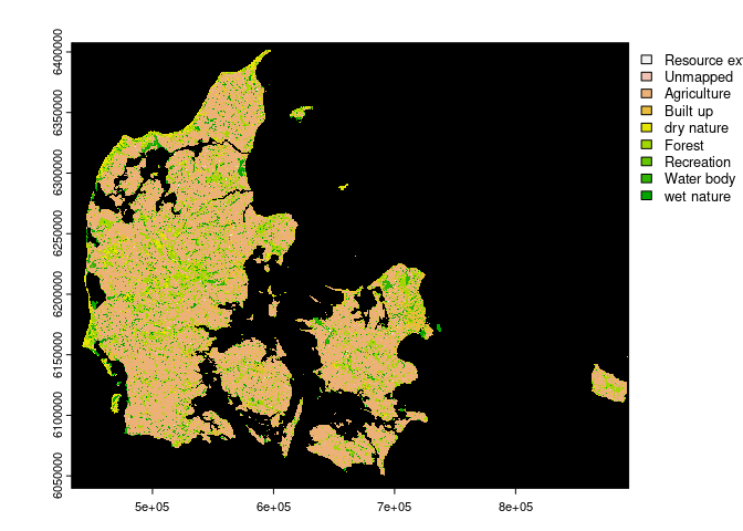
We can see the dry nature type and wet nature type of Denmark in figure 2.1

Figure 2.1: Areas in denmark bellonging to dry and wet nature

Now we can use the calculate_prop to calculate the proportion of each landuse in a certain radius, as an example we will use a radius of 200 meters to calculate the proportions of the nature raster created above, optionally, you can decide which landuses to calculate by using the argument Vars:

proportions <- calculate_prop(Rast = nature, 
                              Radius = 200, 
                              Vars = c("Agriculture", "Forest"))
#> Starting to generate dummy stack [1/3]
#> Calculating the weight matrix [2/3]
#> Generating final stack [3/3]
#> 
|---------|---------|---------|---------|
=========================================

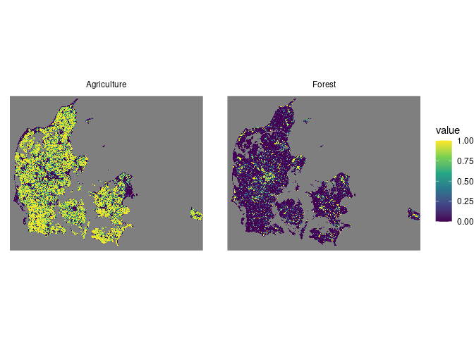
We can see the result in figure 2.2

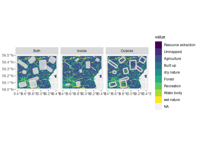
Figure 2.2: Prportion of different habitat types within Denmark

2.2 Summarise data from polygons

This is a function that is very useful to get dataset for shapefiles, the dataset is delivered as proportion of the chosen area that has a particular landuse. There are three types of analysis for this: Inside the polygons, Outside the polygon, and finally inside an outside the polygon, in figure

data(Polygons)
data("Landuse_DK")
Landuse <- terra::unwrap(Landuse_DK)

v <- vect(Polygons, "polygons", crs = terra::crs(Landuse))

Figure 2.3: Showing the summary for some simulated polygons inside, outside, and both

As it can be seen, now the polygons can overlap

2.2.1 Inside the polygons

Test <- summarise_polygons(Rast = Landuse, Polygons = v,
                           Vars = c("Agriculture","Forest"))
#> Using option = inside

Agriculture	Forest
0.6039312	0.2157248
0.8775385	0.0381538
0.5605780	0.2782512
0.7852426	0.1004881
0.7750973	0.0630350
0.4416529	0.3385124
0.7544332	0.0581369
0.5909091	0.3315508
0.3793361	0.3222678
0.4157738	0.1976190

Table 2.1: Proportions for the polygons for agriculture and forest

2.2.2 Inside and outside the polygon

TestBoth <- summarise_polygons(Rast = Landuse, Polygons = v,
                               Vars = c("Agriculture","Forest"), 
                               type = "Both", dist = 2500)
#> Using option = Both

Agriculture	Forest
0.5604590	0.2162687
0.7971613	0.0568796
0.5581856	0.2807765
0.7598044	0.1049355
0.6603998	0.1182466
0.3187107	0.4529922
0.7548519	0.0765115
0.6477639	0.1825726
0.5842719	0.2396753
0.4760104	0.2141929

2.2.3 Outside the polygon

TestOut <- summarise_polygons(Rast = Landuse, 
                              Polygons = v,
                              Vars = c("Agriculture","Forest"), 
                              type = "Outside", dist = 2500)
#> Using option = Outside

Agriculture	Forest
0.5514466	0.2163814
0.7826027	0.0604342
0.5573128	0.2816978
0.7483896	0.1069312
0.6413641	0.1241902
0.2710496	0.4973728
0.7530962	0.0902942
0.6531282	0.1685166
0.6608587	0.2088096
0.4951853	0.2332008