GCP-Big-Data-ML

Notes for the Google Cloud Platform Big Data and Machine Learning Fundamentals course.

https://www.coursera.org/learn/gcp-big-data-ml-fundamentals/home/welcome

https://console.cloud.google.com

WEEK 1

1. Google Cloud Architecture

-----------------------------------------
        2. Big Data/ML Products
-----------------------------------------
 1. Compute Power | Storage | Networking
-----------------------------------------
           0. Security
-----------------------------------------

-2. Abstract away scaling, infrastructure

-1. Process, store, and deliver pipelines, ML models, etc.

-0. Auth

2. Creating a VM on Compute Engine

2.1 Setting up the VM

https://cloud.google.com
Compute --> Compute Engine --> VM Instances
Create a new VM

3.1 Allow full access to cloud APIs

3.2 Since we will access the VM through SSH, we don't need to allow HTTP or HTTPS traffic

Click SSH to connect

At this stage, the new VM has no software.

We can just install stuff like normal:

sudo apt-get install git

(APT: advanced package tool, package manager)

2.2 Sample earthquake data

After installing git, we can pull down the data from our repo:

git clone https://www.github.com/GoogleCloudPlatform/training-data-analyst

Course materials are in:

training-data-analyst/courses/bdml_fundamentals

Go to the Earthquake sample in earthquakevm.

The ingest.sh shell script contains the script to ingest data (less ingest.sh). This script basically just deletes existing data and then wgets a new CSV file containing the data.

Now, transform.py contains a Python script to parse the CSV file and create a PNG from it using matplotlib ( matplotlib notes).

(File details)

Run ./install_missing.sh to get the missing Python libraries, and run the scripts mentioned above to get the CSV and generate the image.

2.3 Transferring the data to bucket storage

Now, since we have generated the image. Let's get it off the VM and delete the VM.

To do this, we need to create some storage: Storage > Storage > Browser > Create Bucket

Now, to view our bucket, we can use:

gsutil ls gs://[bucketname] (hence why bucket names need to be globally unique)

To copy out data to the bucket, we can use:

gsutil cp earthquakes.* gs://[bucketname]

2.4 Stopping/deleting the VM

So now we're finished with our VM, we can either:

STOP Stop the machine. You will still pay for the disk, but not the processing power.

DELETE Delete the machine. You won't pay for anything, but obviously you will lose all of the data.

2.5 Viewing the assets

Now, we want to make our assets in storage publically available. To do this: Select Files > Permissions > Add Members > allUsers > Grant Storage Object Viewer role.

Now, you can use the public link to view your assets.

3. Storage

There are 4 storage types:

Multiregional: Optimized for geo-redundancy, end-user latency
Regional: High performance local access (common for data pipelines you want to run, rather than give global access)
Nearline: Data accessed less than once a month
Coldline: Data accessed less than once a year

4. Edge Network (networking)

Edge node receives the user's request and passes to the nearest Google data center.

Consider node types (Hadoop):

Master node: Controls which nodes perform which tasks. Most work is assigned to...
Worker node: Stores data and performs calculations
Edge node: Facilitate communication between users and master/worker nodes

Edge computing: brings data storage closer to the location where it's needed. In contrast to cloud computing, edge computing does decentralized computing at the edge of the network.

Edge Node (aka. Google Global Cache - GGC): Points close to the user. Network operators and ISPs deploy Google servers inside their network. E.g., YouTube videos could be cached on these edge nodes.

Edge Point of Prescence: Locations where Google connects its network to the rest of the internet.

https://peering.google.com/#/

5. Security

Use Google IAM, etc. to provide security.

BigQuery data is encrypted.

6. Big Data Tool History

GFS: Data can be stored in a distributed fashion
MapReduce: Distributed processing, large scale processing across server clusters. Hadoop implementation
BigTable: Record high volume of data
Dremel: Breaks data into small chunks (shards) and compresses into columnar format, then uses query optimizer to process queries in parallel (service auto-manages data imbalances and scale)
Colossus, TensorFlow: And more...

(Note on Columnar Databases)

Consider typical row-oriented databases. The data is stored in a row. This is great when you want to query multiple columns from a single row.

However, what if you want to get all of the data from all rows from a single column?

For this, we need to read every row, picking out just the columns we want. For example, we want the average age of all the people. This will be slower in row-oriented databases, because even an index on the age column wouldn't help. The DB will just do a sequential scan.

Instead we can store the data column-wise. How does it know which columns to join together into a single set? Each column has a link back to the row number. Or, in terms of implementation, each column could be stored in a separate file. Then, each column for a given row is stored at the same offset in a given file. When you scan a column and find the data you want, the rest of the data for that record will be at the same offset in the other files.

Row oriented

RowId 	EmpId 	Lastname 	Firstname 	Salary
001 	10 	    Smith 	    Joe      	40000
002 	12 	    Jones 	    Mary 	    50000
003 	11 	    Johnson 	Cathy 	    44000
004 	22 	    Jones 	    Bob 	    55000

Column oriented

10:001,12:002,11:003,22:004;
Smith:001,Jones:002,Johnson:003,Jones:004;
Joe:001,Mary:002,Cathy:003,Bob:004;
40000:001,50000:002,44000:003,55000:004;

In terms of IO improvements, if you have 100 rows with 100 columns, it will be the difference between reading 100x2 vs. 100x100.

It also becomes easier to horizontally scale -- make a new file to store more of that column.

It is also easier to add a column -- just add a new file.

Lab 1

Public datasets

Go to BigQuery > Resources > Add Data > Explore public datasets to add publically available datasets.

You can query the datasets using SQL syntax:

SELECT
  name, gender,
  SUM(number) AS total
FROM
  `bigquery-public-data.usa_names.usa_1910_2013`
GROUP BY
  name, gender
ORDER BY
  total DESC
LIMIT
  10

Before you run the query, the query validator in the bottom right will show much data is going to be run.

Creating your own dataset

Resources seem to have the following structure:

Resources > Project > Dataset > Table

To add your own dataset:

Resources > click Project ID > Create dataset (For example babynames)

Then, we can add a table to this dataset.

Click dataset name > Create table

Source > upload from file
File format > CSV
Table name > names_2014
Schema > name:string,gender:string,count:integer

Creating the table will run a job. The table will be created after the job completes.

Click preview to see some of the data.

Then you can query the table like before.

SQL Syntax for BigQuery: https://cloud.google.com/bigquery/docs/reference/standard-sql/

7. GCP Approaches

Google Cloud Platform applications:

Compute Engine: Infrastructure as a service. Run virtual machines on demand in the cloud.
Google Kubernetes Engine (GKE): Clusters of machines running containers (code packages with dependencies)
App Engine: Platform as a service (PaaS). Run code in the cloud without worrying about infrastructure.
Cloud Functions: Serverless environment. Functions as a service (FaaS). Executes code in response to events.

App Engine: long-lived web applications that auto-scale to billions of users.

Cloud functions: Code triggered by event, such as new file uploaded.

Serverless

Although this can mean different things, typically it now means functions as a service (FaaS). I.e., application code is hosted by a third party, eliminating need for server and hardware management. Applications are broken into functions that are scaled automatically.

8. Recommendation Systems

A recommendation system requires 3 things:

Data
Model
Training/serving infrastructure

Point: Train model on data, not rules.

RankBrain

ML applied to Google search. Rather than use heuristics (e.g., if in California and q='giants', show California giants), use previous data to train ML model and display results.

Building a recommendation system

Ingest existing data (input and output, e.g., user ratings of tagged data)
Train model to predict output (e.g., user rating)
Provide recommendation: rate all of the unrated products, show top n.

Ratings will be based on:

Who is this user like?
Is this a good product? (other ratings?)
Predicted rating = user-preference * item-quality

Models can typically be updated once a day or once a week. It does not need to be streaming. Once computed, the recommendations can be stored in Cloud SQL.

So compute the ratings use a batch job (Dataproc), and store them in Cloud SQL.

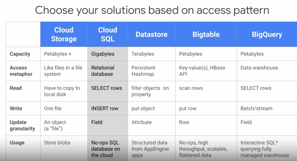
Storage systems

Roughly:

Cloud Storage: Global file system (unstructured)
Cloud SQL: Relational database (transactional/relational data accessed through SQL) (structured/transactional) 2.1 Cloud Spanner: Horizontal scalability (+ more than a few GBs, need a few DBs)
Datastore: Transactional, NoSQL object-oriented database (structured/transactional)
Bigtable: High throughput, NoSQL, append-only data (not transactional) (millisecond latency analytics)
BigQuery: SQL data warehouse to power analytics (seconds latency analytics)

Hadoop Ecosystem

Hadoop: MapReduce framework (HDFS)
Pig: Scripting language that can be compiled into MapReduce jobs
Hive: Data warehousing system and query language. Makes data on distributed file system look like an SQL DB.
Spark: Lets you run queries on your data. Also ML, etc.

Storage

HDFS is used for working storage -- storage during the processing of the job. But all input and output data will be stored in Cloud Storage. So because we store data off-cluster, the cluster only has to be available for a run of the job.

(Recall, you can shut down the compute nodes when not using them, so save your data in Cloud Storage, etc., instead of in the computer node disk.)

Lab 2

Creating Cloud SQL DBs

First, let's create a Cloud SQL instance to hold all of the recommendation data:

SQL > Create Instance > MySQL > Instance ID = 'rentals'

Now the script creates 3 tables:

Accomodation: Basic details
Rating: 1-to-many for accomodation to ratings and user-to-ratings
Recommendation: This will be populated by the recommendation engine

Connect to this instance > Connect using Cloud Shell

An sql connect command will prepopulate to connect to the DB, so you can now run commands as required.

Use show databases; to show the registered DBs.

Run the script to create the recommendation_spark database and underlying tables.

Ingesting Data

Now, before we can populate the Cloud SQL tables we just created, we need to stage the CSV files containing the data on Cloud Storage. To do this, we can either use Cloud Shell commands or the Console UI.

Using Console UI:

Storage > Browser > Create Bucket > Upload CSV files

Now, click the Import function on the Cloud SQL page to populate the SQL tables from the CSV files.

After querying the SQL tables to make sure they populated correctly, type Exit to exit.

Dataproc

Now we will ue Dataproc to train the ML model based on previous ratings.

We need to launch Dataproc and configure it so each machine in the cluster can access Cloud SQL.

Dataproc let you provision Apache Hadoop clusters.

After provisioning your cluster, run a bash script to patch each machine so that its IP is authorized to access the Cloud SQL instance.

Copy over the Python recommendation model.

You edit code via Cloud Shell by using: cloudshell edit train_and_apply.py

Now run the job via Dataproc:

Dataproc console > Jobs > Submit job > Enter file containing job code/set parameters

The job will run through to populate the recommendations.

9. BigQuery

Petabyte data warehoue. Two services in one:

SQL Query Engine (serverless -- fully managed)
Managed data storage
Pay for data stored and queries run, or flat tier
Analysis engine: takes in data and run analysis/model building
Can connect to BigQuery from other tools

Sample Query

Cloud console > Big Query > Create dataset > Create table (can upload from storage, etc.)

When writing queries, use the following format:

FROM [project (name? or id?)].[dataset].[table]

E.g.:

SELECT COUNT(*) AS total_trips
FROM `bigquery-public-data.san_francisco_bikeshare.bikeshare_trips`

(Click on this query to view the table info)

Click the down arrow > Run selected to just run the selected part of the query

Architecture

----------------------------                          ----------------------------
  BigQuery Storage Service    <-- Petabit network -->   BigQuery Query Service
----------------------------                          ----------------------------
 Project                                                 Run queries
   Dataset A | Dataset B                                 Connectors to other products
   Table 1   | Table 1*                                  
   Table 2   | ...
   ...       |
----------------------------                          ----------------------------
 * Tables stored as compressed 
   column in Colossus
 * Supports steams or data ingest

BigQuery Tips

Ctrl/cmd-click on table name: view table
In details, click on field name to insert it into the query
Click More > Format to automatically format the query
Explore in Data Studio > visualize data
Save query > Save query data in project
CREATE OR REPLACE TABLE [dataset].[tablename] AS [SQL QUERY] to save the data into a table, saving you having to rerun the query every time
In the above, you could replace TABLE with VIEW, to just store the query itself. Helpful if the data is changing a lot.

Cloud Dataprep

Provides data on data quality. Provides data cleansing, etc.

10. SQL Array and Structs

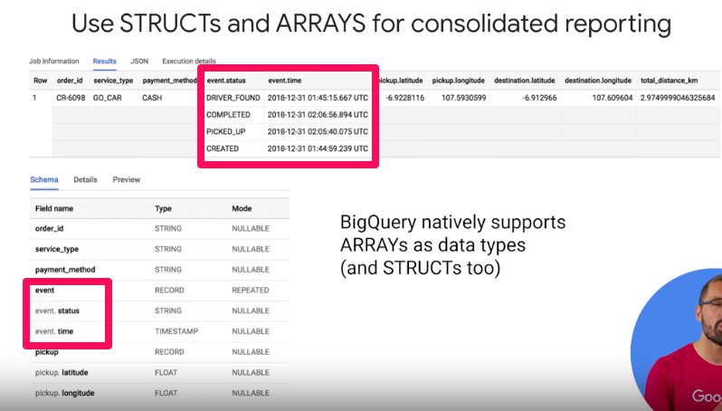
Splitting the data into different tables requires joins or, possibly, denormalization.

To avoid this, we can use two features:

SQL Structs (Records)

These are a datatype that is essentially a collection of fields. You can think of it like a table inside another table.

Array Datatype

Lets you have multiple fields associated with a single row.

11. ML Model

Some terms...

Instance/observation: A row of data in the table
Label: Correct answer known historically (e.g., how much this customer spent), in future data this is what you want to know
Feature columns: Other columns in the table (i.e., used in model, but you don't want to predict them)
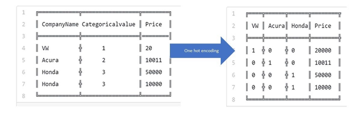
One hot encoding: Turning enums into a matrix of 1s so a not to skew the model

BigQuery ML (BQML)

In BigQuery, we can build models in SQL.

First, build the model in SQL:

CREATE MODEL numbikes.model
OPTIONS
(model_type='linear_reg', labels=['num_trips']) AS
WITH bike_data AS
(
SELECT COUNT(*) a num_trims,
...

Second, write a SQL prediction query:

SELECT predicted_num_trips, num_trips, trip_date
FROM
ml.PREDICT(MODEL 'numbikes.model...

BigQuery's SQL models will:

Auto-tune learning rate
Auto-splits data into training and test (though these hyperparameters can be set manually too)

Process

The general process looks like this:

Get data into BigQuery
Preprocess features (select features) -- create training set
Create model in BigQuery (CREATE MODEL)
Evaluate model
Make predictions with model (ML.predict)

BQML Cheatsheet

Label: Alias a column as 'label', or specify column(s) in OPTIONS using input_label_cols (reminder: labels are what is currently known in training data, but what you want to predict)
Feature: Table columns used as SQL SELECT statement (SELECT * FROM ML.FEATURE_INFO(MODEL ``mydataset.mymodel``) to get info about that column after model is trained)
Model: An object created in BigQuery that resides in BigQuqery dataset
Model Types: Linear regression (predict on numeric field), logistic regression (discrete class -- high or low, spam not spam, etc.) (CREATE OR REPLACE MODEL <dataset>.<name> OPTIONS(model_type='<type>') AS <training dataset>)
Training Progress: `SELECT * FROM ML.TRAINING_INFO(MODEL ``mydataset.mymodel```
Inspect Weights: SELECT * FROM ML.WEIGHTS(MODEL ``mydataset.mymodel``, (<query>))
Evaluation: `SELECT * FROM ML.EVALUATE(MODEL mydataset.mymodel)
Prediction: SELECT * FROM ML.PREDICT(MODEL ``mydataet.mymodel``, (<query>))

Lab 3

Get the conversion rate:

WITH visitors AS(
SELECT
COUNT(DISTINCT fullVisitorId) as total_visitors
FROM `data-to-insights.ecommerce.web_analytics`
),

purchasers AS(
SELECT
COUNT(DISTINCT fullVisitorId) as total_purchasers
FROM `data-to-insights.ecommerce.web_analytics`
WHERE totals.transactions IS NOT NULL
)

SELECT
total_visitors,
total_purchasers,
total_purchasers/total_visitors as conversion_rate
FROM visitors, purchasers

Find the top 5 selling products:

SELECT
p.v2ProductName,
p.v2ProductCategory,
SUM(p.productQuantity) AS units_sold,
ROUND(SUM(p.localProductRevenue/1000000),2) AS revenue
FROM `data-to-insights.ecommerce.web_analytics`,
UNNEST(hits) AS h,
UNNEST(h.product) AS P
GROUP BY 1,2
ORDER BY revenue DESC
LIMIT 5;

This query:

Creates a table containing a row for all of hits UNNEST(hits)
Creates a table containing all of the products in hits UNNEST(h.product)
Select the various fields
Groups by product name and product category

The UNNEST keyword takes an array and returns a table with a single row for each element in the array. OFFSET will help to retain the ordering of the array.

SELECT *
FROM UNNEST(['foo', 'bar', 'baz', 'qux', 'corge', 'garply', 'waldo', 'fred'])
  AS element
WITH OFFSET AS offset
ORDER BY offset;

+----------+--------+
| element  | offset |
+----------+--------+
| foo      | 0      |
| bar      | 1      |
| baz      | 2      |
| qux      | 3      |
| corge    | 4      |
| garply   | 5      |
| waldo    | 6      |
| fred     | 7      |
+----------+--------+

GROUP BY 1,2 refers to the first and second items in the select list.

Analytics schema:

https://support.google.com/analytics/answer/3437719?hl=en

Create the model

CREATE OR REPLACE MODEL `ecommerce.classification_model`
OPTIONS
(
model_type='logistic_reg', # Since we want to classify as A/B
labels = ['will_buy_on_return_visit'] # Set the thing we want to predict
)
AS

#standardSQL
SELECT
  * EXCEPT(fullVisitorId) 
FROM

  # features
  (SELECT
    fullVisitorId,
    IFNULL(totals.bounces, 0) AS bounces,
    IFNULL(totals.timeOnSite, 0) AS time_on_site
  FROM
    `data-to-insights.ecommerce.web_analytics`
  WHERE
    totals.newVisits = 1
    AND date BETWEEN '20160801' AND '20170430') # train on first 9 months
  JOIN
  (SELECT
    fullvisitorid,
    IF(COUNTIF(totals.transactions > 0 AND totals.newVisits IS NULL) > 0, 1, 0) AS will_buy_on_return_visit
  FROM
      `data-to-insights.ecommerce.web_analytics`
  GROUP BY fullvisitorid)
  USING (fullVisitorId)
;

After running, the query will create a new ML model in project:dataset.model

EXCEPT will return all of the rows in the left query not in the right query.

For example:

  WITH a AS (
SELECT * FROM UNNEST([1,2,3,4]) AS n

    ), b AS (
SELECT * FROM UNNEST([4,5,6,7]) AS n)

SELECT * FROM a

EXCEPT DISTINCT

SELECT * FROM b

-- | n |
-- | 1 |
-- | 2 |
-- | 3 |

Evaluate the model

One feature we can use to evaluate the model is the receiver operating characteristic (ROC). Essentially this shows the quality of a binary classifier by mapping true positive rates against false positive rates.

We want to get the area under the curve as close as possible to 1.0

https://cdn.qwiklabs.com/GNW5Bw%2B8bviep9OK201QGPzaAEnKKyoIkDChUHeVdFw%3D

SELECT
  roc_auc,
  CASE
    WHEN roc_auc > .9 THEN 'good'
    WHEN roc_auc > .8 THEN 'fair'
    WHEN roc_auc > .7 THEN 'not great'
  ELSE 'poor' END AS model_quality
FROM
  ML.EVALUATE(MODEL ecommerce.classification_model,  (

SELECT
  * EXCEPT(fullVisitorId)
FROM

  # features
  (SELECT
    fullVisitorId,
    IFNULL(totals.bounces, 0) AS bounces,
    IFNULL(totals.timeOnSite, 0) AS time_on_site
  FROM
    `data-to-insights.ecommerce.web_analytics`
  WHERE
    totals.newVisits = 1
    AND date BETWEEN '20170501' AND '20170630') # eval on 2 months
  JOIN
  (SELECT
    fullvisitorid,
    IF(COUNTIF(totals.transactions > 0 AND totals.newVisits IS NULL) > 0, 1, 0) AS will_buy_on_return_visit
  FROM
      `data-to-insights.ecommerce.web_analytics`
  GROUP BY fullvisitorid)
  USING (fullVisitorId)

));

roc_auc is a queryable field

Improving the model

We can improve the model by adding more features:

CREATE OR REPLACE MODEL `ecommerce.classification_model_2`
OPTIONS
  (model_type='logistic_reg', labels = ['will_buy_on_return_visit']) AS

WITH all_visitor_stats AS (
SELECT
  fullvisitorid,
  IF(COUNTIF(totals.transactions > 0 AND totals.newVisits IS NULL) > 0, 1, 0) AS will_buy_on_return_visit
  FROM `data-to-insights.ecommerce.web_analytics`
  GROUP BY fullvisitorid
)

# add in new features
SELECT * EXCEPT(unique_session_id) FROM (

  SELECT
      CONCAT(fullvisitorid, CAST(visitId AS STRING)) AS unique_session_id,

      # labels
      will_buy_on_return_visit,

      MAX(CAST(h.eCommerceAction.action_type AS INT64)) AS latest_ecommerce_progress,

      # behavior on the site
      IFNULL(totals.bounces, 0) AS bounces,
      IFNULL(totals.timeOnSite, 0) AS time_on_site,
      totals.pageviews,

      # where the visitor came from
      trafficSource.source,
      trafficSource.medium,
      channelGrouping,

      # mobile or desktop
      device.deviceCategory,

      # geographic
      IFNULL(geoNetwork.country, "") AS country

  FROM `data-to-insights.ecommerce.web_analytics`,
     UNNEST(hits) AS h

    JOIN all_visitor_stats USING(fullvisitorid)

  WHERE 1=1
    # only predict for new visits
    AND totals.newVisits = 1
    AND date BETWEEN '20160801' AND '20170430' # train 9 months

  GROUP BY
  unique_session_id,
  will_buy_on_return_visit,
  bounces,
  time_on_site,
  totals.pageviews,
  trafficSource.source,
  trafficSource.medium,
  channelGrouping,
  device.deviceCategory,
  country
);

Point: Ensure you use the same training data. Otherwise differences could be due to differences in input, rather than model improvements.

Now we have a better model, we can make predictions.

Make predictions

SELECT
*
FROM
  ml.PREDICT(MODEL `ecommerce.classification_model_2`,
   (

WITH all_visitor_stats AS (
SELECT
  fullvisitorid,
  IF(COUNTIF(totals.transactions > 0 AND totals.newVisits IS NULL) > 0, 1, 0) AS will_buy_on_return_visit
  FROM `data-to-insights.ecommerce.web_analytics`
  GROUP BY fullvisitorid
)

  SELECT
      CONCAT(fullvisitorid, '-',CAST(visitId AS STRING)) AS unique_session_id,

      # labels
      will_buy_on_return_visit,

      MAX(CAST(h.eCommerceAction.action_type AS INT64)) AS latest_ecommerce_progress,

      # behavior on the site
      IFNULL(totals.bounces, 0) AS bounces,
      IFNULL(totals.timeOnSite, 0) AS time_on_site,
      totals.pageviews,

      # where the visitor came from
      trafficSource.source,
      trafficSource.medium,
      channelGrouping,

      # mobile or desktop
      device.deviceCategory,

      # geographic
      IFNULL(geoNetwork.country, "") AS country

  FROM `data-to-insights.ecommerce.web_analytics`,
     UNNEST(hits) AS h

    JOIN all_visitor_stats USING(fullvisitorid)

  WHERE
    # only predict for new visits
    totals.newVisits = 1
    AND date BETWEEN '20170701' AND '20170801' # test 1 month

  GROUP BY
  unique_session_id,
  will_buy_on_return_visit,
  bounces,
  time_on_site,
  totals.pageviews,
  trafficSource.source,
  trafficSource.medium,
  channelGrouping,
  device.deviceCategory,
  country
)

)

ORDER BY
  predicted_will_buy_on_return_visit DESC;

WEEK 2

Data Pipelines

Ingesting real-time data poses a number of challenges:

Have to scale in real time
Have to deal with data being late
Have to deal with bad data coming in real time (duplicates, missing data, etc.)

Cloud Pub/Sub

Distributed messaging system to handle real-time messaging.

--------------------------------------------------------------------------------------------------------------------

   (sensor data, etc.) > Cloud Pub/Sub > Cloud Dataflow > BigQuery/Cloud Storage > Exploration/Visualization Apps
                         [Ingests data,   [Subscribes to
                          publishes to      Cloud Pub/Sub]
                          subscribers
--------------------------------------------------------------------------------------------------------------------

Serverless Big Data Pipeline

Cloud Pub/Sub Architecture

Cloud Pub/Sub uses topics. These are like channels that is publishes. Subscribers can listen to these topics and pick up messages that are published.

For example:

Setup Pub/Sub with a topic called "HR"
When a new worker joins, the HR system publishes a "NEW HIRE" event to the "HR" topic
Then, downstream applications (facilities, badge activation system) who are subscribed to this topic can get the message and take action as appropriate

Cloud Dataflow

Apache Beam

Used to implement batch or streaming data processing jobs.
Pipelines written in Java, Python, or Go
Creates a model representation of code which is portable across many runners
Runners pass models to an execution environment, which can run on many different engines (e.g., Spark, Cloud Dataflow)
Transformations can be done in parallel, making pipelines scalable

Workflow with Cloud Dataflow

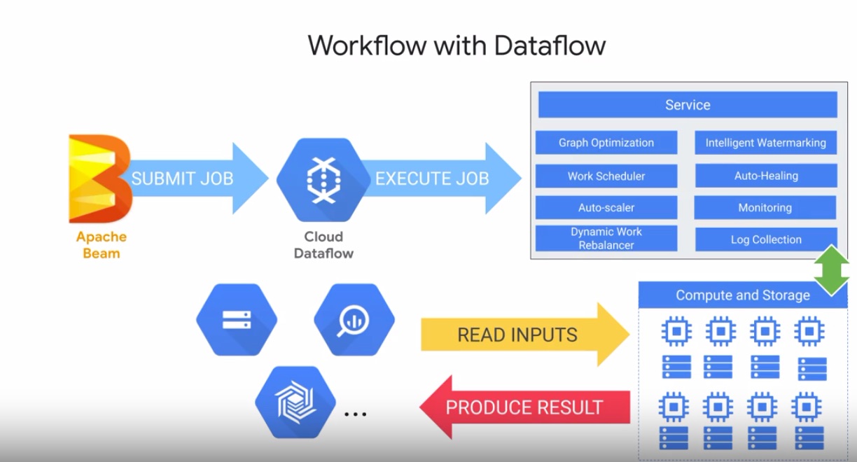
Write code to create model in Beam
Beam passes a job to Cloud Dataflow
Once it receives it, Cloud Dataflow's service:

Optimizes execution graph
Schedules out to workers in distributed fashion
Auto-heal if workers encounter errors
Connect to data sinks to produce results (e.g., BigQuery)

A number of template pipelines are available:

https://github.com/googlecloudplatform/dataflowtemplates

Data Studio

Provides data visualization
Data is live, not just a static image
Click Explore in Data Studio in BigQuery

Creating a report

Create new report
Select a data source (can have multiple data sources)
Create charts: click and draw

Data Studio uses Dimensions and Metric chips.

Dimensions: Categories or buckets of information (area code, etc.). Shown in green.
Metric: Measure dimension values. Measurements, aggregations, count, etc. Shown in blue.

Use calculated fields to create your own metrics.

Lab 1

Cloud Pub/Sub topics

Cloud Pub/Sub lets decouples senders and receivers. Senders send messages to a Cloud Pub/Sub topic, and receivers subscribe to this topic.

_Create a BigQuery dataset

Messages published into Pub/Sub will be stored in BigQuery.

In Cloud Shell, run bq mk taxirides to create a dataset called taxirides in BigQuery
Now create a table inside the dataset:

bq mk \
--time_partitioning_field timestamp \
--schema ride_id:string,point_idx:integer,latitude:float,longitude:float,\
timestamp:timestamp,meter_reading:float,meter_increment:float,ride_status:string,\
passenger_count:integer -t taxirides.realtime

Create a Cloud Storage bucket

Storage > Create Bucket
Name must be globally unique (e.g., project id)

Setup Cloud Dataflow Pipeline

Navigation > Dataflow
Create job from template
Type > Cloud Pub/Sub topic to BigQuery template
Input topic > projects/pubsub-public-data/topics/taxirides-realtime
Output table > qwiklabs-gcp-72fdadec78efe24c:taxirides.realtime
Temporary location > gs://qwiklabs-gcp-72fdadec78efe24c/tmp/
Click run job

Cloud Dataflow will now show a visualization of the Dataflow job running.

Analyze streaming data

You can check the data in BigQuery:

SELECT * FROM taxirides.realtime LIMIT 10;

See aggregated per/minute ride data:

WITH streaming_data AS (

SELECT
  timestamp,
  TIMESTAMP_TRUNC(timestamp, HOUR, 'UTC') AS hour,
  TIMESTAMP_TRUNC(timestamp, MINUTE, 'UTC') AS minute,
  TIMESTAMP_TRUNC(timestamp, SECOND, 'UTC') AS second,
  ride_id,
  latitude, 
  longitude,
  meter_reading,
  ride_status,
  passenger_count
FROM
  taxirides.realtime
WHERE ride_status = 'dropoff'
ORDER BY timestamp DESC
LIMIT 100000

)

# calculate aggregations on stream for reporting:
SELECT 
 ROW_NUMBER() OVER() AS dashboard_sort,
 minute,
 COUNT(DISTINCT ride_id) AS total_rides,
 SUM(meter_reading) AS total_revenue,
 SUM(passenger_count) AS total_passengers
FROM streaming_data
GROUP BY minute, timestamp

Explore in Data Studio

Click Explore in Data Studio
Set up dimensions and metrics as desired

Once finished, stop the Cloud Dataflow pipeline job.

Approaches to ML

Use pre-built AI

Lack enough data to build your own model

Add custom models

Requires 100,000~millions of records of sample data

Create new models

Use pre-built ML building blocks. E.g., https://console.cloud.google.com/vision/ For example, use vision API to extract text and translate API to tranlate it.

AutoML

Use to extend the capabilities of the AI building block without code. For example, extend Vision API to recognize cloud types by uploading photos of clouds with type labels. A confusion matrix shows the % of labels that were correctly/incorrectly labelled.

Uses neural architecture search to build several models and extract the best one.

Lab 2

Get an API key

APIs and Services > Credentials > Create Credentials > API Key

In Cloud Shell, set the API Key as an environment variable:

export API_KEY=<YOUR_API_KEY>

Create storage bucket

Storage > Create bucket >

Make the bucket publically available:

gsutil acl ch -u AllUsers:R gs://qwiklabs-gcp-005f9de6234f0e59/*

Then click the public link to check it worked.

Create JSON request

You can use Emacs in Cloud Shell:

emacs
c-X c-F to create file (this finds file, but type in the file name you want to create and it will create it as an empty buffer)
c-X c-C to save file and kill terminal

(nano seems to work better in Cloud Shell)

Send the request

Use curl to send the request:

curl -s -X POST -H "Content-Type: application/json" --data-binary @request.json https://vision.googleapis.com/v1/images:annotate?key=${API_KEY}

Now, the response will provide some labels based on the pretrained model, but what if we want the model to be able to detect our own labels? In that case, we can feed in some of our own training data. To do this custom training, we can use AutoML.

AutoML

Once setup, AutoML will create a new bucket with the suffix -vcm.

Bind a new environment variable to this bucket:

export BUCKET=<YOUR_AUTOML_BUCKET>

Copy over the training data:

gsutil -m cp -r gs://automl-codelab-clouds/* gs://${BUCKET}

Now we need to set up a CSV file that tells AutoML where to find each image and the labels associated with each image. We just copy it over:

gsutil -m cp -r gs://automl-codelab-clouds/* gs://${BUCKET}

Now copy the file to your bucket:

gsutil cp ./data.csv gs://${BUCKET}

Now, back in the AutoML Vision UI, click New Dataset > clouds > Select a CSV file on Cloud Storage > Create Dataset

The images will be imported from the CSV. After the images have been imported, you can view them and check their labels, etc. You can also change the labels, etc.

(You want at least 100 images for training.)

Click train to start training.

After the model has finished training, you can check the accuracy of the model:

Precision: What proportion of +ve identifications were correct?
Recall: What propotion of actual +ves was identified correctly? (1.0 = good score)

Generating Predictions

Now that we've training our model, we can use it to make some predictions on unseen data.

Go to the Predict tab
Unload images to see predictions

Building a Custom Model

There are threes ways to build custom models in GCP:

Using SQL models
AutoML
ML Engine Notebook (Jupyter) (can write own model with Keras)

Further Courses

From Data to Insights
Data Engineering
ML on GCP
Adv ML on GCP

dexi154/GCP-Big-Data-ML

GCP-Big-Data-ML

WEEK 1

1. Google Cloud Architecture

2. Creating a VM on Compute Engine

2.1 Setting up the VM

2.2 Sample earthquake data

2.3 Transferring the data to bucket storage

2.4 Stopping/deleting the VM

2.5 Viewing the assets

3. Storage

4. Edge Network (networking)

5. Security

6. Big Data Tool History

(Note on Columnar Databases)

Lab 1

7. GCP Approaches

8. Recommendation Systems

Lab 2

9. BigQuery

10. SQL Array and Structs

11. ML Model

Lab 3

WEEK 2

Data Pipelines

Cloud Pub/Sub

Cloud Dataflow

Data Studio

Lab 1

Approaches to ML

AutoML

Lab 2

Building a Custom Model

Further Courses