Soviet dogs in space

Davide Fucci 2020-05-25

The data is provided by Duncan Geere. It is a database of dogs that flew on space missions based on the book Soviet Space Dogs.

Loading basic things. Beside tidyverse, lubridate helps to work with dates, janitor helps linting dataframes, whereas ggforce and ggtext put ggplot on steroids.

dogs <- read_csv("data/Dogs-Database.csv")
flights <- read_csv("data/Flights-Database.csv")

The Dogs dataframe is the most important, contains name of the dogs, gender, and they flight they were on. The flight table contains additional information on the flight (most importantly, altitute).

dogs_tidy <- dogs %>% 
  clean_names() %>% 
  separate_rows(flights, sep = ",") %>% 
  mutate(date_flight = ymd(flights),
         date_death = case_when(str_sub(fate, 1, 4) == "Died" ~ str_sub(fate, 6, 15)),
         date_death = ymd(date_death),
         flight_fate = case_when(date_flight == date_death ~ "Died",
                          TRUE ~ "Survived")) %>% 
  select(-notes, -fate, -flights)

Tidy up the dogs dataframe, linting the column names to use camel case (clean_names()), separate multiple flights in the same cell over several columns, and parse dates. Finally, remove unimportant columns.

flights_tidy <- flights %>% 
  clean_names() %>% 
  select(date_flight = date, rocket, altitude_km, result, notes_flight = notes) %>% 
  filter(altitude_km != "unknown") %>% 
  mutate(altitude = case_when(str_detect(altitude_km, "^[0-9]") ~ parse_number(altitude_km), 
                              str_detect(altitude_km, "orbital") ~ 2000))  # 2000 km is the terrestrial orbit altitude according to Wikipedia

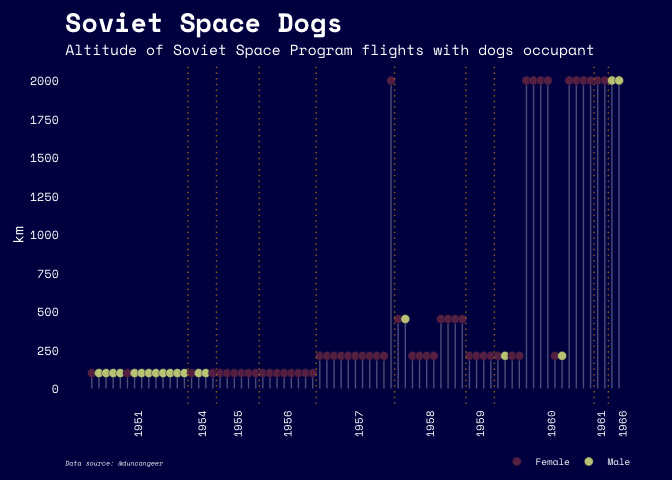
Same for cleaning for flights. Important thing to do here is to parse altitude, as sometimes contains an integer value (in km), other times the string orbital, and other times unknown (which are filtered out).

all_dogs_flights <- dogs_tidy %>% 
  inner_join(flights_tidy, by = "date_flight") %>% 
  mutate(flight_year = year(date_flight)) %>% 
  arrange(date_flight) 
  
all_dogs_flights <- all_dogs_flights %>% 
  mutate(rank = 1:nrow(all_dogs_flights)) # adds incremental rank based on year

Join the two tables, extract only the year of the flight in a separate column which is used as a label for the x-axis in the plot. Order the flights by year and add an incremental id (rank) to use as x-axis value in the plot.

H\T to David Smale for how to clean this dataset. Check his other awesome visualization of Soviet Dogs in Space.

labels = rep("",75) 
to_keep<-c(7,16,21,28,38,48,55,65,72,75) # middle-point within each year range
labels[to_keep] = all_dogs_flights$flight_year[to_keep] 
year_change = c(14.5, 18.5, 24.5, 32.5, 43.5, 53.5, 57.5, 71.5, 73.5) # x-axis value indicating when there is a change in year. For example, there are 14 flights in the first year of data, 4 for the second (14+4=18) and so on.

A bit hackish, but needed to keep only few of the label to avoid to repetitively print the year on the x-axis for each datapoint. year_change are the y=0 intercepts to be plotted.

p <- ggplot(all_dogs_flights, aes(x=rank, y=altitude)) +
  geom_segment(aes(x=rank, y=0, xend=rank, yend=altitude), color="white", alpha = 0.3) +
  geom_point(aes(fill=gender), shape = 21, colour = "#000050", size = 3, stroke = 0.2) + 
  scale_y_continuous(breaks = seq(0, 2250, 250)) +
  scale_fill_manual(values = c("Male" = "#c5ca85", "Female" = "#682d51")) +
  geom_vline(xintercept = year_change, color="#E69F00", alpha =0.7, linetype="dotted") +
  labs(y = "km", x = "", 
       title = "Soviet Space Dogs",
       subtitle = "Altitude of Soviet Space Program flights with dogs occupant",
       caption = "Data source: @duncangeer") + 
  scale_x_continuous(labels = labels, breaks=seq(1,75,1)) +
  theme(plot.background = element_rect(fill = "#000050", colour = "#000050"),
        panel.background = element_rect(fill = "#000050", colour = "#000050"),
        panel.grid.minor = element_blank(),
        panel.grid.major = element_blank(),
        text = element_text(colour = "white", family = "Space Mono"),
        plot.caption = element_text(color = "white", face = "italic", size = 5, hjust = 0),
        axis.text = element_text(colour = "white"),
        axis.text.x = element_text(size=8, colour ="white", angle = 90 ),
        axis.ticks.x = element_blank(),
        axis.ticks.y = element_blank(),
        plot.title = element_text(face = "bold", size = 20),
        plot.margin = margin(10,20,10,10),
        legend.background = element_rect(fill =  alpha("white", 0.0), colour =  alpha("white", 0.0)),
        legend.key = element_rect(fill = "#000050", colour = "#000050" ),
        legend.direction = "horizontal",
        legend.text = element_text(size=7),
        legend.title = element_blank(),
        legend.position = c(0.86, -0.17))
p

Lollipop plot. The taller the stem, the higher the dog flew into space.

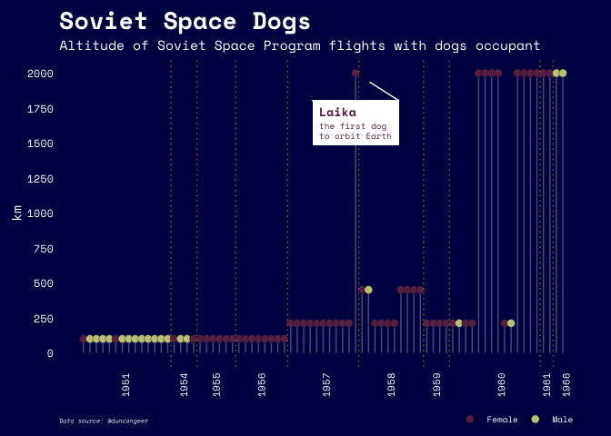
p_annotated <- p + geom_mark_circle(aes(filter = name_latin == 'Laika', label = 'Laika',description = "the first dog\nto orbit Earth"),
                   label.family = "Space Mono",
                   label.fontsize = c(10, 7),
                   label.colour = c("#682d51", "#682d51"),
                   label.fill = "white",
                   label.buffer = unit(1, "mm"),
                   con.colour = "white",
                   colour = NA,
                   con.type = "straight",
                   con.cap = 0)
p_annotated

Annotating the plot with ggtext. See Laika Wikipedia entry.

dfucci/Soviet-Dogs-in-Space

Soviet dogs in space